Introduction
In this post we will be taking a look at the cryptocurrencies Bitcoin (BTC) and Litecoin (LTC). In a previous post we examined price action for BTC, LTC and the LTCBTC ratio. We did this using the Yahoo Finance pricing data extracted using the quantmod package. We then used the powerful plotly package to graph the OHLC (Open High Low Close) pricing data.
In this post we begin with a visual analysis of the OHLC data. We then analyze price movement based on the day of the week. Using this data we apply the non parametric statistical sign test to determine if the proportion of positive to negative price movement is statistically significant. To keep things simple we will only statistically analyze Friday and Sunday. This will help answer the question of whether not the “Friday bump” and “Sunday dump” are real phenomenons or just people’s speculation.
Below we load up the required libraries
library(plotly)
library(ggplot2)
library(quantmod)
library(here)
and then load the required data using the quantmod package. Note that we are cutting off our data collection at the end of June.
# load Bitcoin data
BTC <- getSymbols("BTC-USD", src='yahoo', env=NULL, to="2022-06-30")
names(BTC) <- c("BTC.Open", "BTC.High", "BTC.Low",
                "BTC.Close", "BTC.Volume", "BTC.Adjusted")

# load Litecoin data
LTC <- getSymbols("LTC-USD", src='yahoo', env=NULL, to="2022-06-30")
names(LTC) <- c("LTC.Open", "LTC.High", "LTC.Low",
                "LTC.Close", "LTC.Volume", "LTC.Adjusted")

# load Litecoin price in terms of Bitcoin
LTCBTC <- getSymbols("LTC-BTC", src='yahoo', env=NULL, to="2022-06-30")
names(LTCBTC) <- c("LTCBTC.Open", "LTCBTC.High", "LTCBTC.Low",
                   "LTCBTC.Close", "LTCBTC.Volume", "LTCBTC.Adjusted")
We also load up our Bitcoin and Litecoin halving dates.
BTC_halvings <- read.csv(here('csv', 'crypto', 'july2021',
                              'BTC_halving_dates.csv'))
LTC_halvings <- read.csv(here('csv', 'crypto', 'july2021',
                              'LTC_halving_dates.csv'))
Charts
With our data loaded up we proceed to plotting the OHLC data using candlestick charts. The code is identical to my previous post on cryptocurrencies and will not be shown.
Our plots are made using the plotly package. Below we see Bitcoin’s daily price movement along with its monthly price movement.
We now look at the daily price movement for Litecoin.
Finally we examine the price relationship between Bitcoin and Litecoin using the LTCBTC ratio.
Analysis
With our data visualization complete we want to analyze daily price change. We will look at large scale price change as well as aggregating daily counts of positive and negative price change on a given day. We do this for both Bitcoin and Litecoin, but focus on Bitcoin first.
In the code block below we collect our Bitcoin data into a data frame. With this data we define three additional variables: diff, pc, and weekday. These variables represent the price change during the day, the price percent change during the day and the day of the week as a string respectively.
btc_df <- data.frame(Date=index(BTC),coredata(BTC))

btc_df$diff <- btc_df$BTC.Close - btc_df$BTC.Open
btc_df$pc <- (btc_df$BTC.Close - btc_df$BTC.Open)/ btc_df$BTC.Open
btc_df$weekday <- weekdays(btc_df$Date)
Let’s take a look at our price difference by day for Bitcoin:
ggplot(btc_df, aes(x=Date, y=diff, color=weekday)) +
    ggtitle("BTC Daily Price Change") +
    geom_point()
Notice that most of the variance in the data is coming from recent dates or certain time clusters. Comparing this data to our Bitcoin OHLC chart shows that this variance is related to times when the price of Bitcoin is high.
Below we create a function which takes our Bitcoin data frame btc_df and returns another data frame containing the count of price increases and decreases grouped by day of the week. Note that we have an option for percentile of data to include. This option uses the percent change to determine which data we keep instead of the difference. We will discuss why soon.
sign_aggregator <- function(input, percentile=0){
    days_of_week = c("Sunday", "Monday", "Tuesday", "Wednesday", "Thursday", "Friday", "Saturday")
    df <-data.frame()
    cutoff <- unname(quantile(abs(input$pc), probs = percentile))

    for (day in days_of_week) {
        df <- rbind(df,
              c(
                  day,
                  sum(input[input$weekday == day & abs(input$pc) >= cutoff, ]$diff < 0),
                  sum(input[input$weekday == day & abs(input$pc) >= cutoff, ]$diff > 0)
              )
        )
    }
    colnames(df) <- c("day", "decrease", "increase")
    return(df)
}
In our function we ignore days which have no price change, however:
sum(btc_df$diff == 0)## [1] 0Thus when we include 100% of the data we end up with
(btc_pm_100 <- sign_aggregator(btc_df))## day decrease increase
## 1 Sunday 198 208
## 2 Monday 182 224
## 3 Tuesday 189 217
## 4 Wednesday 199 208
## 5 Thursday 196 211
## 6 Friday 178 228
## 7 Saturday 175 231This, almost surprisingly, indicates that not a single day is more likely to have a price decrease as apposed to a price increase.
With the current data we are may be including very small price changes. Perhaps this is noise and should be removed from consideration. What if we focus on large price changes? This might bias our results with only recent time periods and time clusters with historically high values. Instead we will consider days with significant price movement relative to the current price. For this we will use the percent change formula \[C = \frac{x_2-x_1}{x_1}\] where \(C\) determines the relative change from our initial value \(x_1\) to \(x_2\) to determine which subset of the data we will use.
Let’s take a look at our percent change data for Bitcoin
ggplot(btc_df, aes(x=Date, y=pc, color=weekday)) +
    ggtitle("BTC Daily Price Percent Change") +
    geom_point()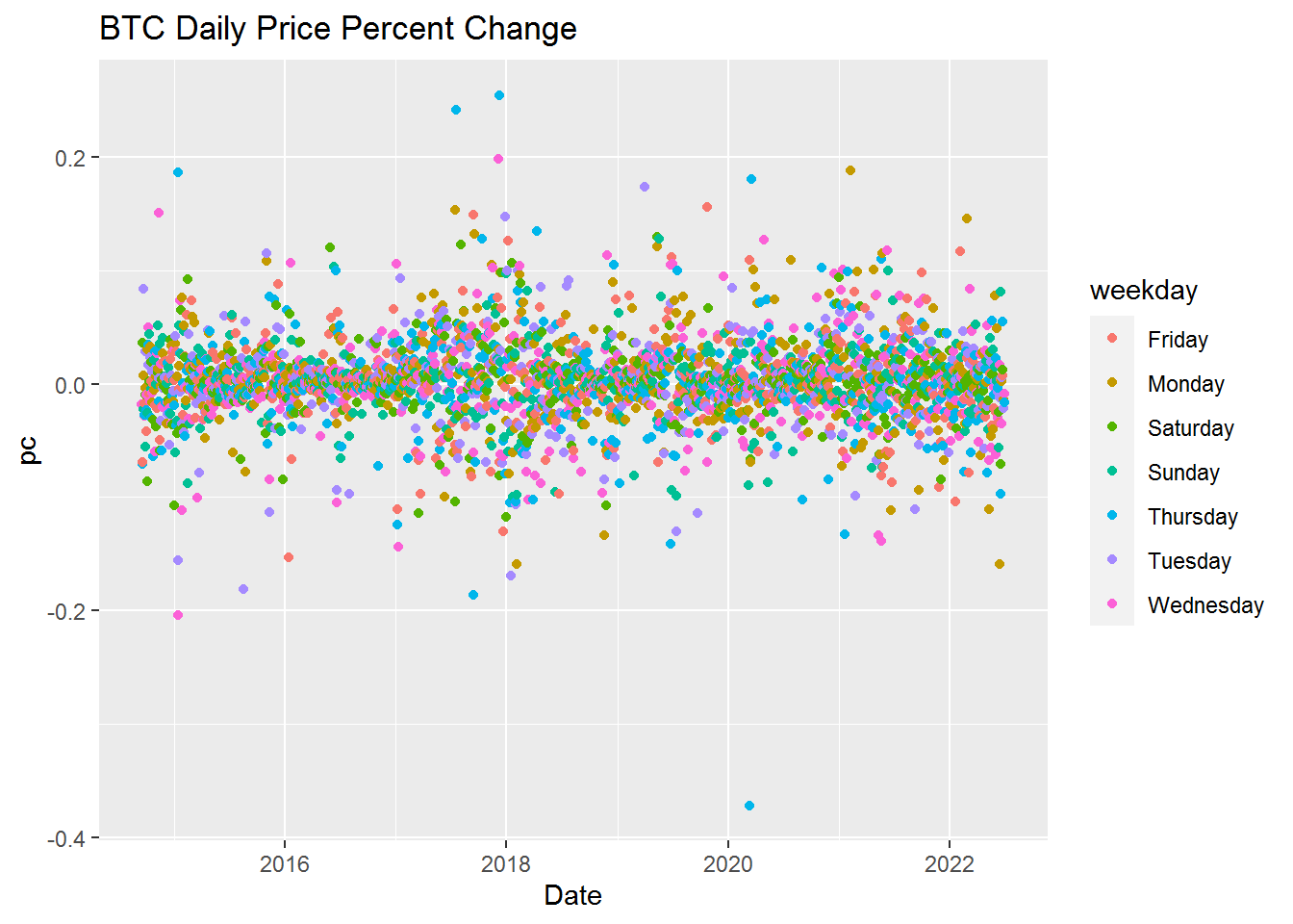
As we can see above the percent change data is more evenly distributed across time.
With our previous observations in mind we will take a look at the top 50% of our data based on the absolute value of the percent change.
(btc_pm_50 <- sign_aggregator(btc_df, 0.5))## day decrease increase
## 1 Sunday 87 95
## 2 Monday 100 124
## 3 Tuesday 98 118
## 4 Wednesday 101 111
## 5 Thursday 103 116
## 6 Friday 91 108
## 7 Saturday 73 97We still have a higher number of price increases appearing than decreases for each day. Though it does appear that certain days of the week may have less volatility since they have fewer overall observations than other days.
For our last look at the Bitcoin data we consider the top 10% of the data and get
(btc_pm_10 <- sign_aggregator(btc_df, 0.9))## day decrease increase
## 1 Sunday 12 12
## 2 Monday 18 34
## 3 Tuesday 22 15
## 4 Wednesday 24 24
## 5 Thursday 24 23
## 6 Friday 22 24
## 7 Saturday 15 16While we can see a slightly different picture forming with this subset of data, we must keep in mind that this data that is significantly different from the average daily price data due to how much data we removed. Still, it is interesting to see Monday having a significantly higher count of price increases and Tuesday with a higher count of price decreases.
Now let’s take a look at Litecoin. As with Bitcoin we create a data frame to hold all the data and then add the variables diff, pc, and weekday.
ltc_df <- data.frame(Date=index(LTC),coredata(LTC))

ltc_df$diff <- ltc_df$LTC.Close - ltc_df$LTC.Open
ltc_df$pc <- (ltc_df$LTC.Close - ltc_df$LTC.Open)/ ltc_df$LTC.Open
ltc_df$weekday <- weekdays(ltc_df$Date)
Below we take a look at our price differences.
ggplot(ltc_df, aes(x=Date, y=diff, color=weekday)) +
    ggtitle("LTC Daily Price Change") +
    geom_point()
Similar to Bitcoin, we can see higher variance during periods which correspond to higher price values. Looking at the percent change we get
ggplot(ltc_df, aes(x=Date, y=pc, color=weekday)) +
    ggtitle("LTC Daily Price Percent Change") +
    geom_point()
This chart seems to indicate a couple interesting differences compared to the Bitcoin percent change graph. First off, we seem to have more outliers and higher variance. Another thing is that the price variance appears higher after around 2017 than before. Asides from these two main observations the data does seem more evenly distributed as compared to the price difference data.
We will now take a look at our data aggregated by price increase and decrease. First we look at all of the data
(ltc_pm_100 <- sign_aggregator(ltc_df, 0))## day decrease increase
## 1 Sunday 210 196
## 2 Monday 217 189
## 3 Tuesday 205 201
## 4 Wednesday 220 187
## 5 Thursday 211 196
## 6 Friday 190 216
## 7 Saturday 199 207We see more decreases in price than increases on Sunday, Monday, Tuesday, Wednesday and Thursday. We see more increases than decreases on Friday and Saturday.
For the most significant 50% of the data based on the absolute value of the percent change we get
(ltc_pm_50 <- sign_aggregator(ltc_df, 0.5))## day decrease increase
## 1 Sunday 99 92
## 2 Monday 113 106
## 3 Tuesday 95 98
## 4 Wednesday 105 97
## 5 Thursday 122 93
## 6 Friday 100 120
## 7 Saturday 71 111Finally for the most significant 10% of the data based on the absolute value of the percent change we get
(ltc_pm_10 <- sign_aggregator(ltc_df, 0.9))## day decrease increase
## 1 Sunday 13 16
## 2 Monday 19 27
## 3 Tuesday 14 23
## 4 Wednesday 25 27
## 5 Thursday 22 24
## 6 Friday 19 28
## 7 Saturday 9 19Ultimately we should be careful about cherry picking our data, but it is interesting to note that when we look at the top 10% of the Litecoin data, based on the absolute value of the percent change, we see that we have more significant price increases on any given day than prices decreases for the same day. This is almost the opposite of the full data set. Perhaps this indicates to some extent that Litecoin slowly goes down in price, but quickly moves up.
Statistical Testing
For our statistical hypothesis testing we will use the full data set. Our goal is to test for Litecoin and Bitcoin if price is more likely to increase on a Friday and also if price is more likely to decrease on a Sunday. In particular, for Friday, using significance level \(\alpha = 0.05\) we test the null hypothesis \[H_0: \textrm{the price is not more likely to go up on a Friday}\] versus the alternative hypothesis \[H_1: \textrm{the price is more likely to go up on a Friday.}\] We also test using significance level \(\alpha = 0.05\) the null hypothesis \[H_0: \textrm{the price is not more likely to go down on a Sunday}\] versus the alternative hypothesis \[H_1: \textrm{the price is more likely to go down on a Sunday.}\]
To test this we use a non-parametric test called the Sign test. Note that we could likely use more powerful test, however, in this case we will stick with this test. Also note that the sign test is a special case of the binomial test when \(p=0.5\). Our results for Bitcoin are below:
# Test whether BTC price increases on Friday
x <- as.numeric(btc_pm_100$increase[6])  # number of successes
y <- as.numeric(btc_pm_100$decrease[6])  # number of fails
n <- x + y

binom.test(x, n, p=0.5, alternative="greater", conf.level=0.95)
##
## Exact binomial test
##
## data: x and n
## number of successes = 228, number of trials = 406, p-value = 0.00746
## alternative hypothesis: true probability of success is greater than 0.5
## 95 percent confidence interval:
## 0.5196016 1.0000000
## sample estimates:
## probability of success
## 0.5615764# Test whether BTC price decreases on Sunday
x <- as.numeric(btc_pm_100$decrease[1]) # number of successes
y <- as.numeric(btc_pm_100$increase[1]) # number of fails
n <- x + y
binom.test(x, n, p=0.5, alternative="greater", conf.level=0.95)##
## Exact binomial test
##
## data: x and n
## number of successes = 198, number of trials = 406, p-value = 0.7074
## alternative hypothesis: true probability of success is greater than 0.5
## 95 percent confidence interval:
## 0.4458158 1.0000000
## sample estimates:
## probability of success
## 0.4876847Which tells us with significance level \(\alpha=0.05\) that we since our p-value is less than \(\alpha\) we can reject the null hypothesis that the price of Bitcoin is not more likely to go up on a Friday in favor of the alternative hypothesis that the price of Bitcoin is more likely to go up on a Friday. On the other hand with significance level \(\alpha=0.05\) we cannot reject the null hypothesis that Bitcoin is not more likely to go down on a Sunday.
Testing for Litecoin we have:
# Test whether LTC price increases on Friday
x <- as.numeric(ltc_pm_100$increase[6])  # number of successes
y <- as.numeric(ltc_pm_100$decrease[6])  # number of fails
n <- x + y

binom.test(x, n, p=0.5, alternative="greater", conf.level=0.95)
##
## Exact binomial test
##
## data: x and n
## number of successes = 216, number of trials = 406, p-value = 0.1073
## alternative hypothesis: true probability of success is greater than 0.5
## 95 percent confidence interval:
## 0.4899803 1.0000000
## sample estimates:
## probability of success
## 0.5320197# Test whether LTC price decreases on Sunday
x <- as.numeric(ltc_pm_100$decrease[1]) # number of successes
y <- as.numeric(ltc_pm_100$increase[1]) # number of fails
n <- x + y
binom.test(x, n, p=0.5, alternative="greater", conf.level=0.95)##
## Exact binomial test
##
## data: x and n
## number of successes = 210, number of trials = 406, p-value = 0.2594
## alternative hypothesis: true probability of success is greater than 0.5
## 95 percent confidence interval:
## 0.4752232 1.0000000
## sample estimates:
## probability of success
## 0.5172414With Litecoin we cannot reject our null hypotheses in either case with a significance level of \(\alpha=0.05\).
Conclusion
Based on our results above we can conclude a few things. Firstly, from a graphical perspective, Litecoin has more significant daily percent change in its price than Bitcoin. Another thing we can see is that the proportion of days in which Bitcoin goes up is higher than the proportion of days in which Litecoin goes. Finally, at least from the simple way this experiment was set up, there is very little evidence of a “Friday bump” and “Sunday dump” in prices. Perhaps with a more sophisticated analysis more evidence could appear. For example instead of considering only if the price went up or down on a given day we could ask if the price goes up on a Friday is there a corresponding price decrease on Sunday. Ultimately, if we consider the question separately, all we can say is that the price tends to go up alot, especially with Bitcoin. So we will leave this exercise as inconclusive for now, but our current analysis does not show any particular evidence of a “Friday bump” and “Sunday dump”.