Introduction
In this post we will look at the total number of Christmas trees harvested in a year as well as well as the total number of operations in a state with tree sales. The data we have is from realchristmastrees.org and includes the years 2002, 2007 and 2012.
Our objective with the data will be to create choropleth maps for each year and each type of data. To accomplish this we use spatial data found here.
The primary packages we will use are shown below.
library(sp)
library(tmap)
library(here)
library(dplyr)
library(magrittr)
library(ggplot2)
library(stringr)
library(tools)
library(pdftools)
Data Cleaning
Our first objective is to load the Christmas tree data and make it usable. Since our original data starts as a pdf we need to carefully inspect it at each step to determine the correct next step. Using pdf_text from the pdftools package we are able to load our data into character vectors of length 2 and 1 for our trees harvested dataset and number of retailer operations dataset respectively.
f1 <- here("csv", "christmas_trees", "trees_harvested.pdf")
trees_harvested <- pdftools::pdf_text(pdf = f1)

f2 <-here("csv", "christmas_trees", "operations_with_sales.pdf")
retailers <- pdftools::pdf_text(pdf = f2)
Below we look at the first element of the trees_harvested dataset. This is the data we need to work with. So we can ignore the second element.
print(trees_harvested[1])## [1] " STATES BY TOTAL TREES HARVESTED\n\n 2012 2007 2002\nTOTAL 17,318,440 17,415,971 20,806,705\nOREGON 6,446,506 6,850,841 6,466,551\nNORTH CAROLINA 4,288,563 3,085,383 2,915,507\nMICHIGAN 1,739,538 1,572,208 2,380,173\nPENNSYLVANIA 1,028,888 1,179,733 1,724,419\nWISCONSIN 611,387 950,440 1,605,981\nWASHINGTON 587,047 785,304 1,164,139\nVIRGINIA 478,069 313,710 507,791\nNEW YORK 274,444 348,043 618,917\nMAINE 195,833 126,908 164,406\nCONNECTICUT 159,091 113,622 133,861\nOHIO 151,327 272,981 372,957\nVERMONT 134,504 168,206 151,249\nNEW HAMPSHIRE 131,876 82,124 107,725\nMINNESOTA 130,527 202,259 463,885\nCALIFORNIA 109,045 119,855 383,940\nTENNESSEE 93,874 166,542 149,770\nINDIANA 89,252 198,899 186,303\nNEW JERSEY 68,471 78,791 132,458\nILLINOIS 65,937 112,617 144,008\nMARYLAND 55,926 77,801 99,183\nMASSACHUSETTS 52,188 75,914 72,522\nGEORGIA 50,112 50,607 80,952\nWEST VIRGINIA 49,867 42,102 60,098\nTEXAS 38,645 42,327 80,914\nSOUTH CAROLINA 35,381 31,113 38,871\nMISSOURI 32,810 27,344 92,483\nIDAHO 27,732 46,145 55,083\nIOWA 27,077 39,575 57,254\nNEBRASKA 22,513 15,160 24,215\nALABAMA 16,355 31,183 35,670\nFLORIDA 16,214 13,776 15,320\nMISSISSIPPI 15,997 20,889 39,594\nRHODE ISLAND 15,962 19,251 23,085\nKANSAS 11,350 15,731 29,094\nLOUISIANA 10,811 17,227 43,742\nMONTANA 9,028 32,104 43,793\nOKLAHOMA 8,760 14,310 18,818\nKENTUCKY 7,987 23,724 56,473\nCOLORADO 7,902 13,404 11,508\nDELAWARE 7,627 10,819 16,183\nARKANSAS 5,806 10,636 18,146\nSOUTH DAKOTA 2,620 4,161 3,715\nUTAH 2,525 2,126 3,744\nHAWAII 2,007 8,323 4,233\nNORTH DAKOTA 735 1,150 2,007\nARIZONA 300 289 (D)\nALASKA 24 0 0\nNEVADA (D) 0 (D)\nNEW MEXICO (D) 314 2,935\nWYOMING 0 0 3,030\n"We can see that the entire pdf table of data in the original dataset has been transformed into a single character string. We will have to do a few different things to get this data into a usable format. Our first step is the remove the new space characters \n and create a new character vector with each line. We do this below and display the first 10 lines.
th_lines <- strsplit(trees_harvested[1], '\n')[[1]]

th_lines %>% head(10) %>% print
## [1] " STATES BY TOTAL TREES HARVESTED"
## [2] ""
## [3] " 2012 2007 2002"
## [4] "TOTAL 17,318,440 17,415,971 20,806,705"
## [5] "OREGON 6,446,506 6,850,841 6,466,551"
## [6] "NORTH CAROLINA 4,288,563 3,085,383 2,915,507"
## [7] "MICHIGAN 1,739,538 1,572,208 2,380,173"
## [8] "PENNSYLVANIA 1,028,888 1,179,733 1,724,419"
## [9] "WISCONSIN 611,387 950,440 1,605,981"
## [10] "WASHINGTON 587,047 785,304 1,164,139"With our slightly cleaner data, we now have each row of our table as a single element in our new character vector. This is a good step, however, the first 4 lines are not really part of our state data. Our next step is to remove the top four rows and then split the character string into four parts corresponding to state, 2002, 2007 and 2012. Since we will have to do something similar for both datasets we create a function below to do this which returns a dataframe. Note that we also remove some confusing characters like (D) and extra commas.
df_from_chr <- function(lines, splits) {
    lines <- lines[- c(1:4)]  # remove first 4 lines
    df <- data.frame()  # create empty dataframe


    # loop over lines to go into dataframe
    for (line in lines) {
        # split lines along splits
        new_row = c(
            substr(line, 1, splits[1]),
            substr(line, splits[1] + 1, splits[2]),
            substr(line, splits[2] + 2, splits[3]),
            substr(line, splits[3] + 3, nchar(line))
        )
        # remove confusing characters
        for (i in 1:4) {
            new_row[i] %<>%
                trimws %>%
                str_replace_all("\\(D\\)", "NA") %>%
                str_remove_all(",")
        }
        df <- rbind(df, new_row)  # add line to dataframe
    }

    # add dataframe names and create numeric columns
    names(df) <- c("State", "2012", "2007", "2002")
    df$`2012` <- as.numeric(unlist(df["2012"]))
    df$`2007` <- as.numeric(unlist(df["2007"]))
    df$`2002` <- as.numeric(unlist(df["2002"]))

    # return value
    df
}
Below we apply our function to the harvested tree dataset using appropriately placed splitting points.
th_df <- df_from_chr(th_lines, c(15, 30, 47))We print our new result below:
print(th_df)## State 2012 2007 2002
## 1 OREGON 6446506 6850841 466551
## 2 NORTH CAROLINA 4288563 3085383 915507
## 3 MICHIGAN 1739538 1572208 380173
## 4 PENNSYLVANIA 1028888 1179733 724419
## 5 WISCONSIN 611387 950440 605981
## 6 WASHINGTON 587047 785304 164139
## 7 VIRGINIA 478069 313710 507791
## 8 NEW YORK 274444 348043 618917
## 9 MAINE 195833 126908 164406
## 10 CONNECTICUT 159091 113622 133861
## 11 OHIO 151327 272981 372957
## 12 VERMONT 134504 168206 151249
## 13 NEW HAMPSHIRE 131876 82124 107725
## 14 MINNESOTA 130527 202259 463885
## 15 CALIFORNIA 109045 119855 383940
## 16 TENNESSEE 93874 166542 149770
## 17 INDIANA 89252 198899 186303
## 18 NEW JERSEY 68471 78791 132458
## 19 ILLINOIS 65937 112617 144008
## 20 MARYLAND 55926 77801 99183
## 21 MASSACHUSETTS 52188 75914 72522
## 22 GEORGIA 50112 50607 80952
## 23 WEST VIRGINIA 49867 42102 60098
## 24 TEXAS 38645 42327 80914
## 25 SOUTH CAROLINA 35381 31113 38871
## 26 MISSOURI 32810 27344 92483
## 27 IDAHO 27732 46145 55083
## 28 IOWA 27077 39575 57254
## 29 NEBRASKA 22513 15160 24215
## 30 ALABAMA 16355 31183 35670
## 31 FLORIDA 16214 13776 15320
## 32 MISSISSIPPI 15997 20889 39594
## 33 RHODE ISLAND 15962 19251 23085
## 34 KANSAS 11350 15731 29094
## 35 LOUISIANA 10811 17227 43742
## 36 MONTANA 9028 32104 43793
## 37 OKLAHOMA 8760 14310 18818
## 38 KENTUCKY 7987 23724 56473
## 39 COLORADO 7902 13404 11508
## 40 DELAWARE 7627 10819 16183
## 41 ARKANSAS 5806 10636 18146
## 42 SOUTH DAKOTA 2620 4161 3715
## 43 UTAH 2525 2126 3744
## 44 HAWAII 2007 8323 4233
## 45 NORTH DAKOTA 735 1150 2007
## 46 ARIZONA 300 289 NA
## 47 ALASKA 24 0 0
## 48 NEVADA NA 0 NA
## 49 NEW MEXICO NA 314 2935
## 50 WYOMING 0 0 3030We now repeat our process for retail operations. Below we look at the data.
print(retailers)## [1] " STATES BY NUMBER OF OPERATIONS WITH SALES\n\n 2012 2007 2002\nTOTAL 12,976.00 13,366.00 14,677.00\nOREGON 1,250 1320 1106\nNORTH CAROLINA 1,151 934 1043\nPENNSYLVANIA 1,079 1205 1326\nNEW YORK 875 844 1001\nMICHIGAN 826 900 1076\nNEW JERSEY 700 884 899\nWISCONSIN 689 849 859\nOHIO 534 594 775\nWASHINGTON 518 534 508\nVIRGINIA 512 352 514\nCONNECTICUT 490 338 382\nMASSACHUSETTS 409 280 306\nCALIFORNIA 328 322 403\nMAINE 310 236 216\nMINNESOTA 276 280 327\nILLINOIS 254 248 338\nVERMONT 232 255 252\nNEW HAMPSHIRE 223 181 173\nINDIANA 189 202 265\nWEST VIRGINIA 179 173 184\nMARYLAND 151 180 204\nSOUTH CAROLINA 149 179 152\nFLORIDA 148 53 79\nIOWA 137 169 215\nGEORGIA 136 144 188\nTENNESSEE 111 179 152\nMISSISSIPPI 110 147 162\nTEXAS 108 254 310\nMISSOURI 105 131 196\nCOLORADO 92 122 91\nKENTUCKY 81 129 143\nIDAHO 79 80 56\nNEBRASKA 77 71 84\nLOUISIANA 74 87 113\nALABAMA 67 59 91\nKANSAS 63 67 102\nRHODE ISLAND 51 49 60\nMONTANA 46 51 54\nARKANSAS 31 51 41\nOKLAHOMA 31 63 73\nDELAWARE 25 41 58\nHAWAII 23 44 19\nUTAH 21 33 26\nSOUTH DAKOTA 13 19 14\nNORTH DAKOTA 12 12 15\nALASKA 3 0 0\nARIZONA 3 0 0\nNEW MEXICO 3 17 20\nNEVADA 2 1 2\nWYOMING 0 3 4\n"Our next step is to remove new line characters \n and print the first 10 rows.
r_lines <- strsplit(retailers, '\n')[[1]]

r_lines %>% head(10) %>% print
## [1] " STATES BY NUMBER OF OPERATIONS WITH SALES"
## [2] ""
## [3] " 2012 2007 2002"
## [4] "TOTAL 12,976.00 13,366.00 14,677.00"
## [5] "OREGON 1,250 1320 1106"
## [6] "NORTH CAROLINA 1,151 934 1043"
## [7] "PENNSYLVANIA 1,079 1205 1326"
## [8] "NEW YORK 875 844 1001"
## [9] "MICHIGAN 826 900 1076"
## [10] "NEW JERSEY 700 884 899"We use our function df_from_chr to split the character rows and create a new dataframe.
r_df <- df_from_chr(r_lines, c(15, 27, 38))We now print our new dataframe and after this we are ready to consider spatial choropleth maps.
print(r_df)## State 2012 2007 2002
## 1 OREGON 1250 1320 1106
## 2 NORTH CAROLINA 1151 934 1043
## 3 PENNSYLVANIA 1079 1205 1326
## 4 NEW YORK 875 844 1001
## 5 MICHIGAN 826 900 1076
## 6 NEW JERSEY 700 884 899
## 7 WISCONSIN 689 849 859
## 8 OHIO 534 594 775
## 9 WASHINGTON 518 534 508
## 10 VIRGINIA 512 352 514
## 11 CONNECTICUT 490 338 382
## 12 MASSACHUSETTS 409 280 306
## 13 CALIFORNIA 328 322 403
## 14 MAINE 310 236 216
## 15 MINNESOTA 276 280 327
## 16 ILLINOIS 254 248 338
## 17 VERMONT 232 255 252
## 18 NEW HAMPSHIRE 223 181 173
## 19 INDIANA 189 202 265
## 20 WEST VIRGINIA 179 173 184
## 21 MARYLAND 151 180 204
## 22 SOUTH CAROLINA 149 179 152
## 23 FLORIDA 148 53 79
## 24 IOWA 137 169 215
## 25 GEORGIA 136 144 188
## 26 TENNESSEE 111 179 152
## 27 MISSISSIPPI 110 147 162
## 28 TEXAS 108 254 310
## 29 MISSOURI 105 131 196
## 30 COLORADO 92 122 91
## 31 KENTUCKY 81 129 143
## 32 IDAHO 79 80 56
## 33 NEBRASKA 77 71 84
## 34 LOUISIANA 74 87 113
## 35 ALABAMA 67 59 91
## 36 KANSAS 63 67 102
## 37 RHODE ISLAND 51 49 60
## 38 MONTANA 46 51 54
## 39 ARKANSAS 31 51 41
## 40 OKLAHOMA 31 63 73
## 41 DELAWARE 25 41 58
## 42 HAWAII 23 44 19
## 43 UTAH 21 33 26
## 44 SOUTH DAKOTA 13 19 14
## 45 NORTH DAKOTA 12 12 15
## 46 ALASKA 3 0 0
## 47 ARIZONA 3 0 0
## 48 NEW MEXICO 3 17 20
## 49 NEVADA 2 1 2
## 50 WYOMING 0 3 4Spatial Data
Now that our data is in a good format for use, we need to load up our spatial data. We do that below.
tree_geo <- here("csv", "christmas_trees",
                 "gadm36_USA_1_sp.rds") %>%
    readRDS()
Taking a look at our spatial data we can see that we are using a class of SpatialPolygonsDataFrame. The dataframe portion of this data contains 51 observations which corresponds to the 50 states of the U.S. as well as the District of Columbia.
str(tree_geo, 2)## Formal class 'SpatialPolygonsDataFrame' [package "sp"] with 5 slots
## ..@ data :'data.frame': 51 obs. of 10 variables:
## ..@ polygons :List of 51
## ..@ plotOrder : int [1:51] 2 44 27 5 32 29 3 23 38 6 ...
## ..@ bbox : num [1:2, 1:2] -179.2 18.9 179.8 72.7
## .. ..- attr(*, "dimnames")=List of 2
## ..@ proj4string:Formal class 'CRS' [package "sp"] with 1 slotOur goal is to combine this spatial dataframe with our two Christmas tree datasets. Below we take a look at four rows of the dataframe in our spatial data. We can see that we have the country name, state name, and whether it is a state or other type of region. The other type of region will corresponds to the District of Columbia.
tree_geo@data[1:4, c("NAME_0", "NAME_1", "ENGTYPE_1")]## NAME_0 NAME_1 ENGTYPE_1
## 1 United States Alabama State
## 12 United States Alaska State
## 23 United States Arizona State
## 34 United States Arkansas StateThe next two steps check whether or not our tree datasets are missing data from our spatial dataframe.
# for th_df

# Determine spelling mismatches between dataframe and
# geographical dataframe missing from or mismatched
# with corresponding regions in tree_geo
excluded_names = c()
for (name in tree_geo$NAME_1){
    if (!(tolower(name) %in% tolower(th_df$State))) {
        excluded_names <- append(excluded_names, name)
    }
}
print(excluded_names)
## [1] "District of Columbia"# for r_df
# Determine spelling mismatches between dataframe and
# geographical dataframe missing from or mismatched
# with corresponding regions in tree_geo
excluded_names = c()
for (name in tree_geo$NAME_1){
if (!(tolower(name) %in% tolower(r_df$State))) {
excluded_names <- append(excluded_names, name)
}
}
print(excluded_names)## [1] "District of Columbia"We can see in both cases we do not have data for the District of Columbia. To resolved this we add to each of our tree dataframes a row containing the missing name along with NA values.
# add NA values as needed for District of Columbia
new_row <- data.frame("District of Columbia", NA, NA, NA)

names(new_row) <- names(th_df)
th_df <- rbind(th_df, new_row)
th_df <- th_df[order(th_df$State),]

names(new_row) <- names(r_df)
r_df <- rbind(r_df, new_row)
r_df <- r_df[order(r_df$State),]
Our next check for each dataframe is to determine if our spatial data and tree dataframes have the same order.
# We determine whether or not tree_geo and our th_df have
# same order for state / region names
incorrect_names <- c()
for (index in 1:length(tree_geo$NAME_1)){
    if (tolower(tree_geo$NAME_1[index]) !=
            tolower(th_df$State[index])) {
        incorrect_names <- append(incorrect_names, th_df$State[index])
    }
}
print(incorrect_names)
## NULL# We determine whether or not tree_geo and our r_df have
# same order for state / region names
incorrect_names <- c()
for (index in 1:length(tree_geo$NAME_1)){
if (tolower(tree_geo$NAME_1[index]) !=
tolower(r_df$State[index])) {
incorrect_names <- append(incorrect_names, r_df$State[index])
}
}
print(incorrect_names)## NULLSince we get NULL for each result we are free to combine each dataframe which we do below.
th_df["State"] <- th_df$State %>% tolower %>% toTitleCase
th_spdf <- SpatialPolygonsDataFrame(Sr=tree_geo, data=th_df, match.ID = FALSE)

r_df["State"] <- r_df$State %>% tolower %>% toTitleCase
r_spdf <- SpatialPolygonsDataFrame(Sr=tree_geo, data=r_df, match.ID = FALSE)
Below we look at our new SpatialPolygonsDataFrame for each category of tree data and are now ready for spatial visualization.
str(th_spdf, 2)## Formal class 'SpatialPolygonsDataFrame' [package "sp"] with 5 slots
## ..@ data :'data.frame': 51 obs. of 4 variables:
## ..@ polygons :List of 51
## ..@ plotOrder : int [1:51] 2 44 27 5 32 29 3 23 38 6 ...
## ..@ bbox : num [1:2, 1:2] -179.2 18.9 179.8 72.7
## .. ..- attr(*, "dimnames")=List of 2
## ..@ proj4string:Formal class 'CRS' [package "sp"] with 1 slot
## ..$ comment: chr "TRUE"str(r_spdf, 2)## Formal class 'SpatialPolygonsDataFrame' [package "sp"] with 5 slots
## ..@ data :'data.frame': 51 obs. of 4 variables:
## ..@ polygons :List of 51
## ..@ plotOrder : int [1:51] 2 44 27 5 32 29 3 23 38 6 ...
## ..@ bbox : num [1:2, 1:2] -179.2 18.9 179.8 72.7
## .. ..- attr(*, "dimnames")=List of 2
## ..@ proj4string:Formal class 'CRS' [package "sp"] with 1 slot
## ..$ comment: chr "TRUE"Visualization
In this section we put everything together and showcase our results. We will look at our results for the harvested tree dataset first for each year and then for the retail operations dataset. Due to the small amount of harvested trees and making the map too stretched we remove Alaska and Hawaii from our results.
condition = th_spdf@data$State != "Alaska" & th_spdf@data$State != "Hawaii"
new_spdf <- th_spdf[condition,]

bbox_new <- sf::st_bbox(new_spdf) # current bounding box

xrange <- bbox_new$xmax - bbox_new$xmin # range of x values
yrange <- bbox_new$ymax - bbox_new$ymin # range of y values

# bbox_new[1] <- bbox_new[1] - (0.5 * xrange) # xmin - left
# bbox_new[3] <- 0.1 * bbox_new[3] # xmax - right
# bbox_new[2] <- bbox_new[2] - (0.5 * yrange) # ymin - bottom
bbox_new[4] <- bbox_new[4] + (0.5 * yrange) # ymax - top

bbox_new <- bbox_new %>%  # take the bounding box ...
  sf::st_as_sfc() # ... and make it a sf polygon

tm_shape(new_spdf, bbox=bbox_new) +
    tm_polygons(col="2002", breaks=c(0, 500, 10000, 100000, 1000000, 5000000, 10000000)) +
    tm_borders(lty="solid") +
    tm_style("cobalt", bg.color="#9CC3CD") +
    tm_layout(frame=FALSE, title="Christmas Trees Harvested\nper State",
            title.size=3,
            legend.title.size=1.5, legend.text.size=1,
            legend.position=c("right", "top"))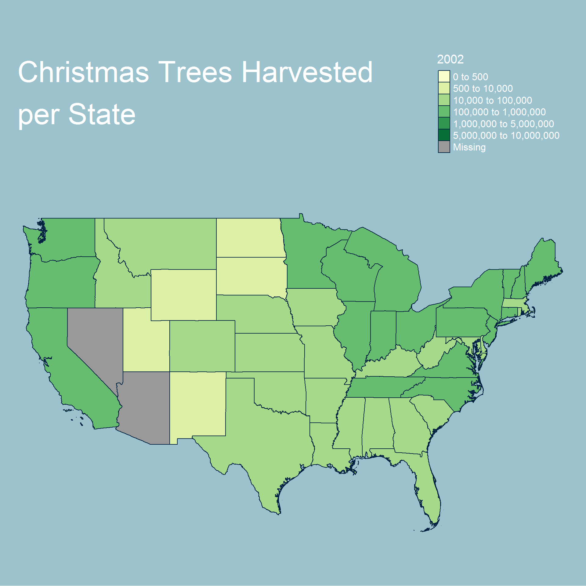
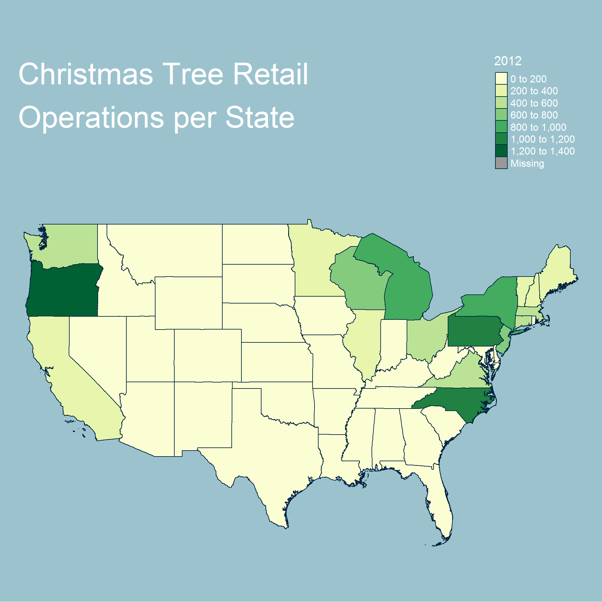
We now look at our values for retail operations.
condition = th_spdf@data$State != "Alaska" & th_spdf@data$State != "Hawaii"
new_spdf <- r_spdf[condition,]

bbox_new <- sf::st_bbox(new_spdf) # current bounding box

xrange <- bbox_new$xmax - bbox_new$xmin # range of x values
yrange <- bbox_new$ymax - bbox_new$ymin # range of y values

# bbox_new[1] <- bbox_new[1] - (0.5 * xrange) # xmin - left
# bbox_new[3] <- 0.1 * bbox_new[3] # xmax - right
# bbox_new[2] <- bbox_new[2] - (0.5 * yrange) # ymin - bottom
bbox_new[4] <- bbox_new[4] + (0.5 * yrange) # ymax - top

bbox_new <- bbox_new %>%  # take the bounding box ...
  sf::st_as_sfc() # ... and make it a sf polygon

tm_shape(new_spdf, bbox=bbox_new) +
    tm_fill("2002") +
    tm_borders(lty="solid") +
    tm_style("cobalt", bg.color="#9CC3CD") +
    tm_layout(frame=FALSE, title="Christmas Tree Retail\nOperations per State",
            title.size=3,
            legend.title.size=1.5, legend.text.size=1,
            legend.position=c("right", "top"))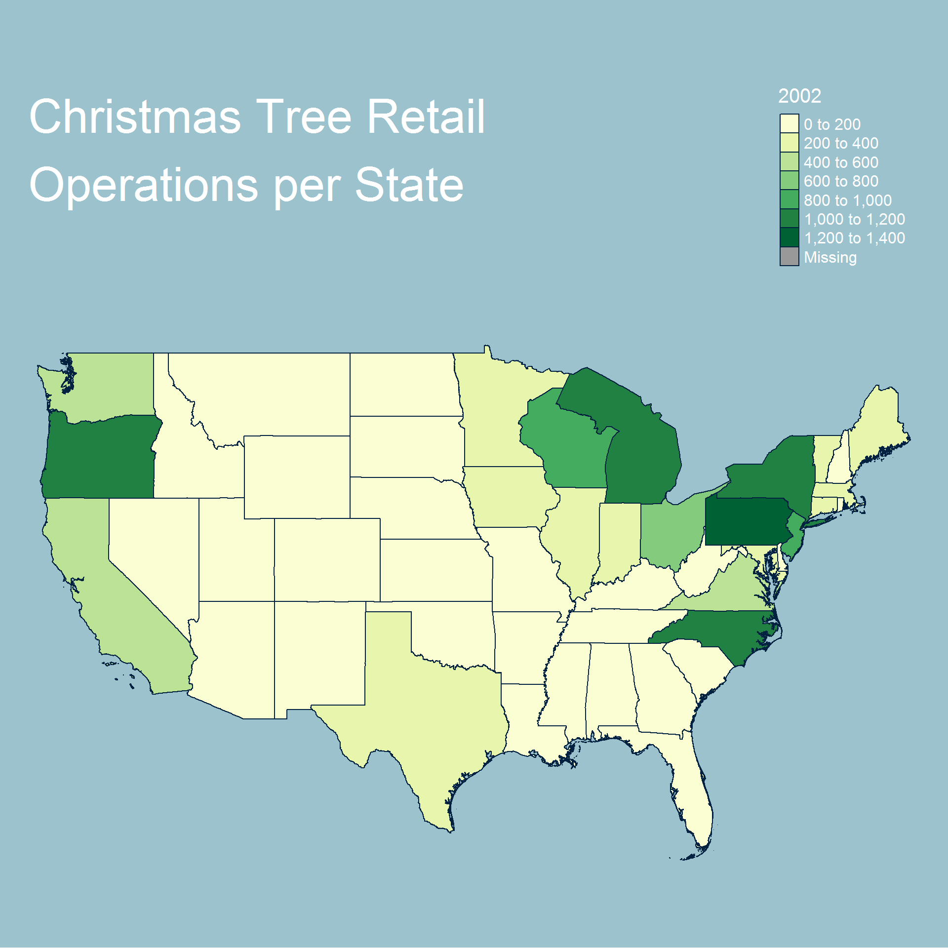

Conclusion
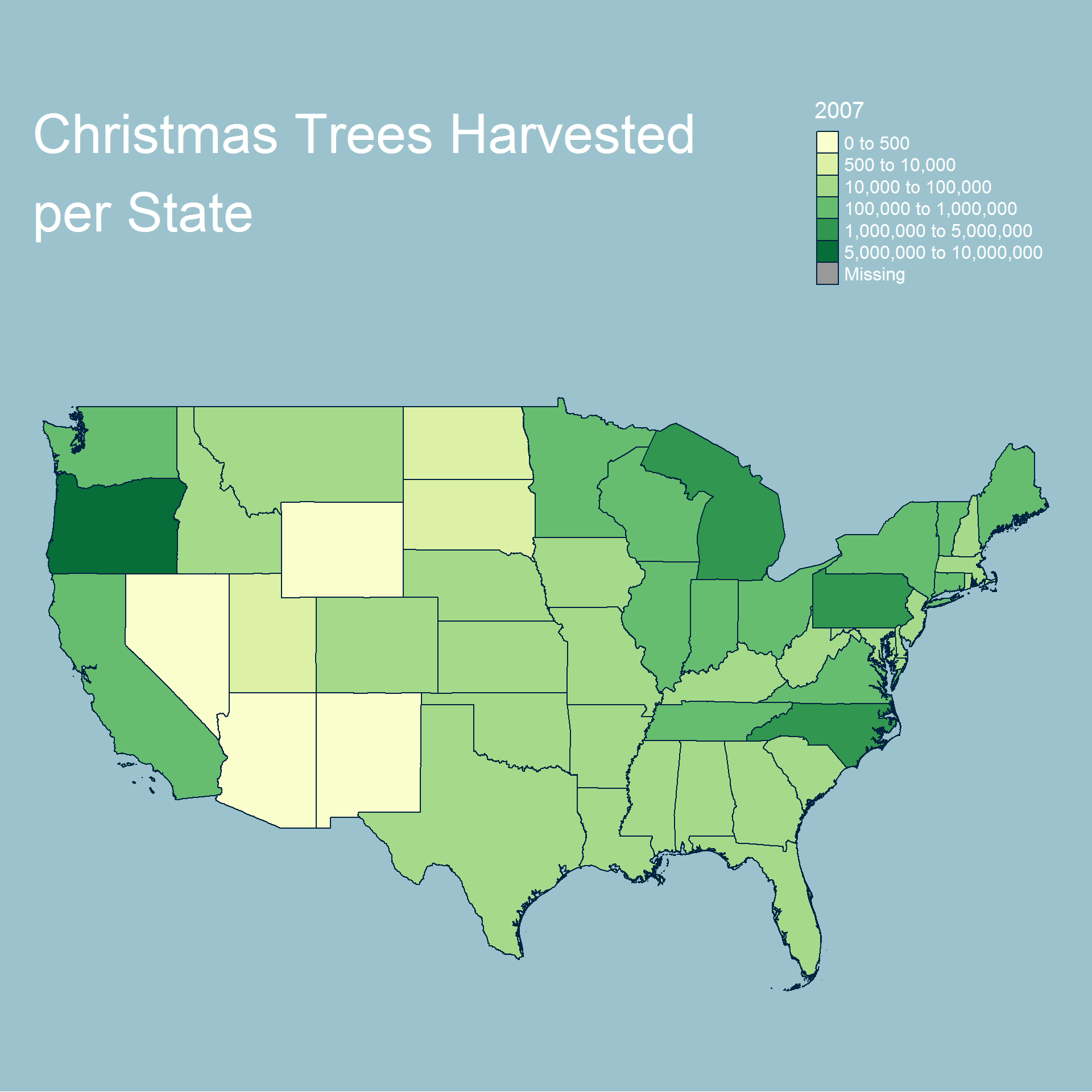
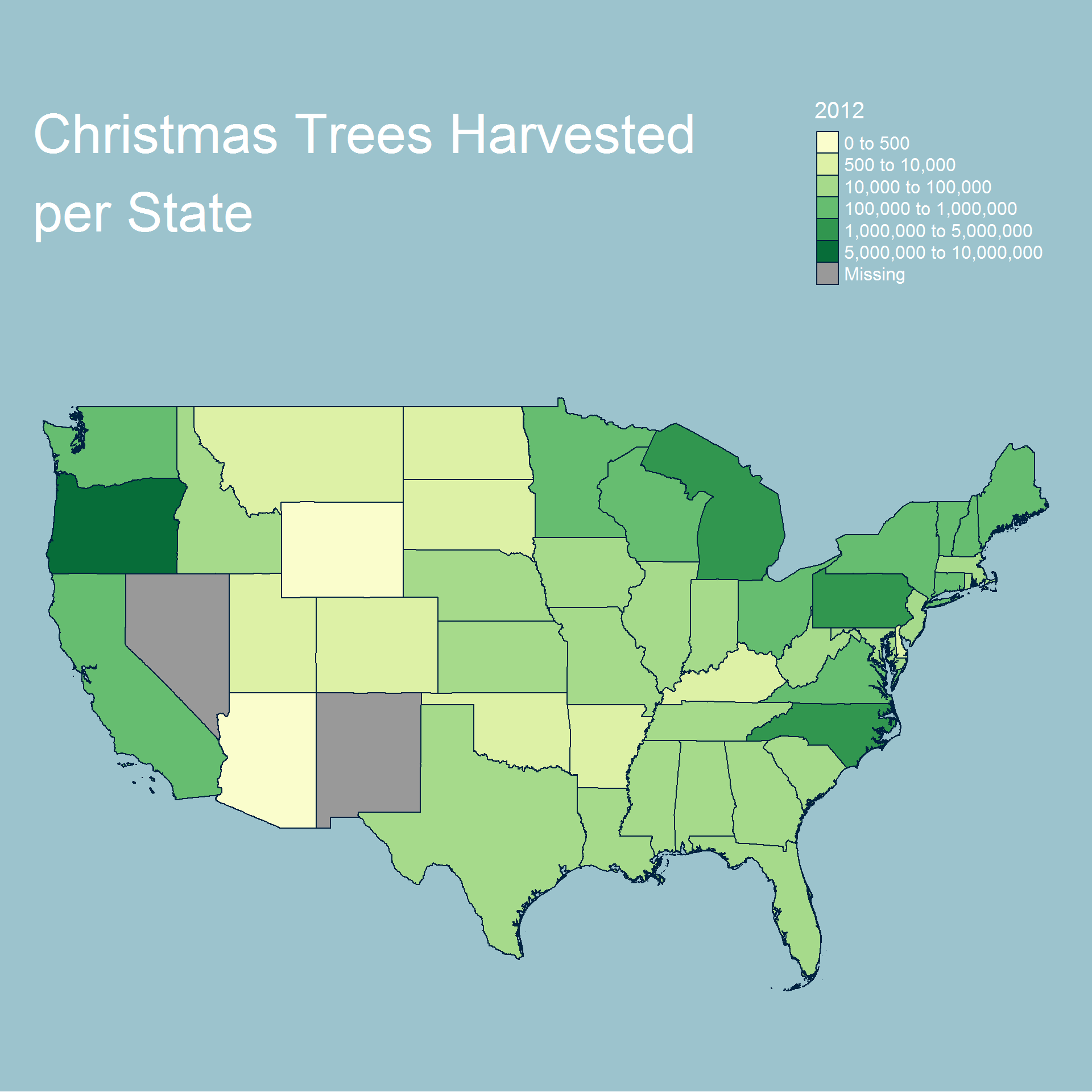
Based on our choropleth maps we can see that the total number of trees being harvested tends to be near the states with large bodies of water. This, however, does not extend to the southern states. We can also see a slight trend over time towards certain states such as Oregon and North Carolina harvesting the most trees.
In terms of retail operations the results are almost identical each year and show that most operations are either in the north east or north west of the country. Similar to the harvested tree dataset we see that Oregon and North Carolina are very prominent in the map.
Overall we can see that most operations and trees are grown either on the east or west coast and generally further north. We also see additional activity near the great lakes.
Further research in this topic could include determining where evergreen trees and species used for Christmas trees naturally grow and what type of climate they grow best in. Additionally, trying to find more recent data could be advantageous. We could also attempt a statistical analysis on the datasets to see if the numbers really are changing significantly between years.