Worlds Largest Pumpkins

Introduction

In this project we examine giant pumpkins. We will use Don Langevin’s Giant Pumpkin website for our data source. The data is a bit messy and will require some data cleaning before it can be used. So this project will be broken up into data cleaning and and then visualization.

Data Cleaning

Before we make our data presentable we load up our primary packages.

library(here)
library(ggplot2)
library(stringr)
library(ggbeeswarm)

With our packages ready we start by reading in our pumpkin dataset which was manually collected from Don Langevin’s Giant Pumpkin website.

pumpkins_raw <- read.csv(here("csv", "largest_pumpkins.csv"))

This dataset includes the 100 largest pumpkins ever recorded at the time this dataset was collected. Below we examine the structure of the dataframe.

str(pumpkins_raw)

## 'data.frame':    100 obs. of  9 variables:
##  $ Pumpkin   : chr  "2702.9 Cutrupi 2021" "2624.6 Willemijns 2016" "2593.7 Paton 2020" "2551.9 Mendi 2020" ...
##  $ State     : chr  "Tuscany" "OV" "England" "Navarre" ...
##  $ Country   : chr  "Italy" "Belgium" "United Kingdom" "Spain" ...
##  $ Seed      : chr  "1885.5 Werner" "2145.5 McMullen 2015" "1875 MENDI \"B\"\"\"" "2183.7 Mendi 2019" ...
##  $ x         : chr  "x" "x" "x" "x" ...
##  $ Pollinator: chr  "Self" "1872 Willemijns 2015" "2005 HAIST" "self" ...
##  $ OTT       : int  514 496 502 485 490 489 493 469 488 490 ...
##  $ Est       : int  2553 2175 2431 2255 2307 2296 2332 2091 2283 2307 ...
##  $ X.....    : int  6 21 7 13 10 10 8 18 7 6 ...

We can see that the pumpkin column actually contains the weight of the pumpkin, the person or team responsible for growing the pumpkin and the year the pumpkin was grown. This will require us to split this column into multiple columns. Another concern, which show’s up for the 28th entry, is teams with more than one word for a name. We see this below.

example_splitting <- pumpkins_raw$Pumpkin[28]
example_splitting

## [1] "2258.6 Willemijns Team 2020"

Before we resolve this problem for the entire dataset we design and implement a solution for just this observation. We start by splitting the string along spaces.

example_split <- unlist(strsplit(example_splitting, " "))
example_split

## [1] "2258.6"     "Willemijns" "Team"       "2020"

This leaves us with two strings in the middle. So our goal is to take the first string for the weight, the last string for the year, and use the remaining strings for the team name. We show our process for this in the code block below.

example_parts <- example_split
example_end <- tail(example_parts, 1)  # get end
example_parts <- head(example_parts, -1)  # remove end
example_start <- example_parts[1]  # get start
example_parts <- tail(example_parts, -1)  # remove start
# combine middle
example_middle <- str_c(example_parts, collapse=" ")

example_start

## [1] "2258.6"

example_middle

## [1] "Willemijns Team"

example_end

## [1] "2020"

With our single observation completed, we reproduce this process for the entire column. This is started by creating vectors to contain the new information.

pumpkins <- pumpkins_raw$Pumpkin

weights <- rep(0, length(pumpkins))
teams <- rep(0, length(pumpkins))
years <- rep(0, length(pumpkins))



for (i in 1:length(pumpkins)){
    pumpkin <- pumpkins[i]
    pumpkin <- unlist(strsplit(pumpkin, " "))
    years[i] <- tail(pumpkin, 1)  # get end
    pumpkin <- head(pumpkin, -1)  # remove end
    weights[i] <- pumpkin[1]  # get start
    pumpkin <- tail(pumpkin, -1)  # remove start
    # combine middle
    teams[i] <- str_c(pumpkin, collapse=" ")
}

With our vectors we create a new dataframe. The reason we are simply creating a new dataframe is that our previous dataframe had some columns which are useless to this project (for example: a column containing only the letter x) and a few other columns which will be avoided. So we create a new dataframe using the extracted Pumpkin column as well as a few other interested columns. We also do a couple additional data cleaning tasks.

pumpkins_clean <- data.frame(
    Weight=as.numeric(weights),
    Team=teams,
    Year=as.integer(years))

pumpkins_clean$State <- pumpkins_raw$State
pumpkins_clean$Country <- pumpkins_raw$Country
pumpkins_clean$OTT <- pumpkins_raw$OTT

# note that both UK and United Kingdoms as well
# as US and United States are used for country names
# we combine these to just UK and US
pumpkins_clean$Country[pumpkins_clean$Country == "United Kingdom"] <- "UK"
pumpkins_clean$Country[pumpkins_clean$Country == "United States"] <- "US"

Even with our clean dataset we still have some missing values. Rather than remove these observations completely we create a second dataframe without the missing values.

no_zero <- pumpkins_clean$OTT != 0
no_na <- !is.na(pumpkins_clean$OTT)
pumpkins_no_outliers <- pumpkins_clean[no_zero & no_na, ]

We have now completed our data cleaning process and are left with a nearly complete dataframe pumpkins_clean and a dataframe with some removed missing values pumpkins_no_outliers.

Visualization

With our data cleaning out of the way we now take a look at the data.

Our first visualizations will focus on Weight by Year. Our very first plot uses a beeswarm plot since our dates have a more categorical nature to them and hence may overlap otherwise.

ggplot(
    pumpkins_no_outliers,
    aes(
        x=as.factor(Year),
        y=Weight,
        color=as.factor(Year))
    ) +
    geom_beeswarm(cex=3) +
    ggtitle("Weight by Year") +
    labs(y="Weight (lbs)", x=NULL, color="Year")

Our second plot is similar, except we use a boxplot instead.

ggplot(
    pumpkins_clean,
    aes(
        y=Weight,
        x=as.factor(Year),
        fill=as.factor(Year))
    ) +
    geom_boxplot() +
    ggtitle("Weight by Year") +
    labs(y="Weight (lbs)", x=NULL, fill="Year")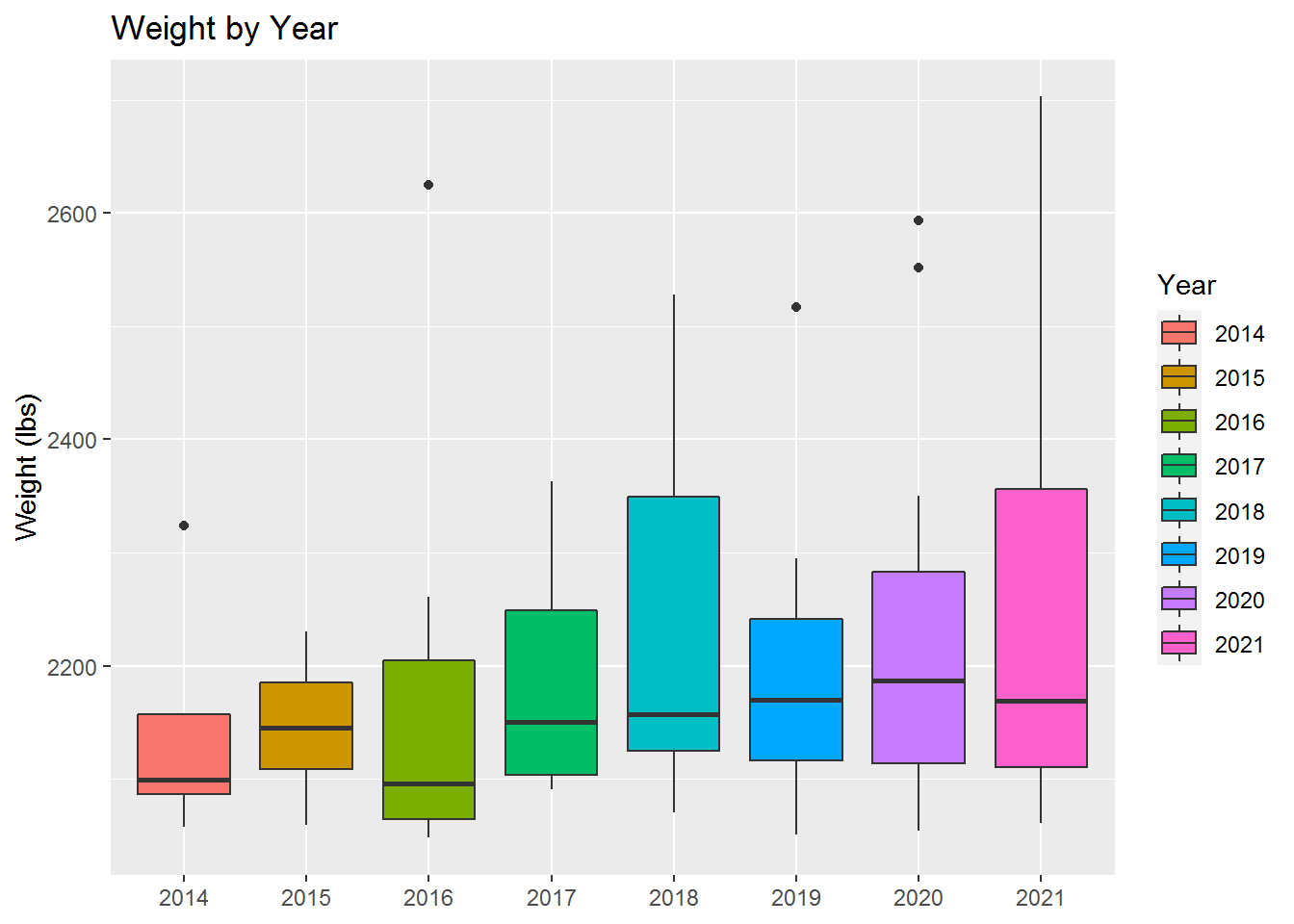

From the beeswarm plot we can see a general increase in the quantity of top 100 pumpkins as the year becomes closer to the present. And from both plots we can see a general trend showing heavier pumpkins being grown in the most recent years.

We now examine the pumpkins by which countries grow the heaviest pumpkins.

ggplot(
    pumpkins_clean,
    aes(y=Weight, x=Country, fill=Country)
    ) +
    geom_boxplot() +
    ggtitle("Weight by Country") +
    labs(y="Weight (lbs)", x=NULL)

Based on our boxplot we can see that only a few countries are represented. Italy and Spain having perhaps the most impressive results. Since this doesn’t indicate the quantity, however, we will also display a beeswarm plot as we did above.

ggplot(
    pumpkins_clean,
    aes(y=Weight, x=Country, color=Country)
    ) +
    geom_beeswarm(cex=2) +
    ggtitle("Weight by Country") +
    labs(y="Weight (lbs)", x=NULL)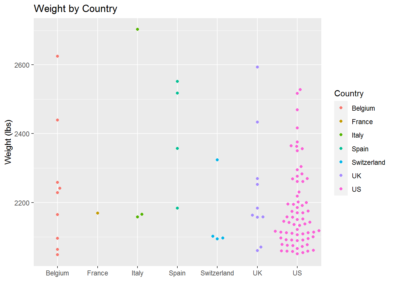

This chart really adds to the previous plot by showing us that the United States, by far, has the most top 100 heaviest pumpkins. It also shows very clearly that Italy has the heaviest pumpkin ever grown. It also shows that Spain’s results include a couple great pumpkins, but does not have quantities in line with countries like Belgium, the United Kingdoms and the United States.

For our last visualization we examine OTT plotted against Weight. What is OTT? It is a measurement used by big pumpkin growers to estimate the weight of a pumpkin. OTT itself stands for Over The Top. We examine below if OTT appears to be a good method for estimating a pumpkins weight.

ggplot(
    pumpkins_no_outliers,
    aes(x=OTT, y=Weight, color=Year)
    ) +
    geom_point() +
    ggtitle("Weight by OTT Measure") +
    labs(y="Weight (lbs)", x="OTT (in)")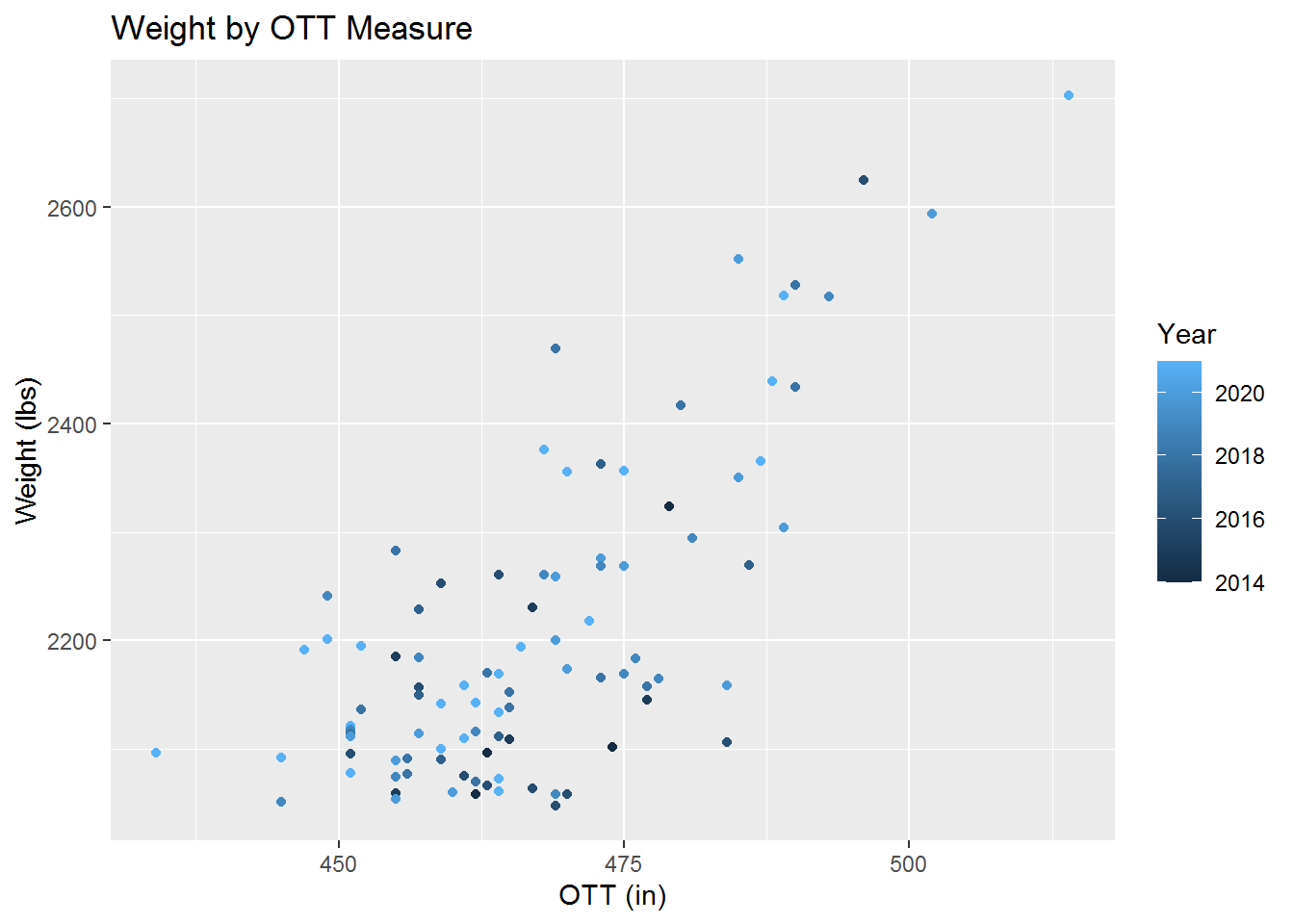

Based on the above scatter plot it would appear the OTT is reasonably good, but certainly not a replacement for weighing the pumpkin. Testing for linear correlation we get a correlation between OTT and Weight below.

cor(pumpkins_no_outliers$Weight, pumpkins_no_outliers$OTT)

## [1] 0.73635

This value basically agrees with our above observation by indicating we have some linear correlation. Perhaps there is a better model than linear for the relationship, but the spread of the data indicates not much would likely be gained. Overall OTT seems like a good method for estimating pumpkin weight while the pumpkin is still growing and cannot be properly weighed.

Conclusion

This is a neat dataset which gives us a good idea of recent pumpkin records, however, there is plenty more we could explore in the world of giant pumpkins. One thing we could look into is the world record pumpkin weights through the years. It also is worth congratulating Cutrupi for their world record 2021 pumpkin of 2702.9 lbs. That is truly impressive!