Introduction
In this post we take a brief look at the most popular programming languages. Our data is from Kaggle and was originally derived from the PYPL PopularitY of Programming Language Index. The values we will work with represent percentage share of search results. The assumption from PYPL is that the more often a programming language is searched the more popular it is. The search values are derived from Google Trends.
In this project we will rely on the xts package to create some simple, but illustrative graphs.
library(here)
library(xts)
Once our packages our loaded we load our data.
tpl <- read.csv(here("csv", "kaggle_2021_sept", "top-prog-lang04-21.csv"))A cursory glance at the data shows that we have 207 observations and 29 variables.
str(tpl)## 'data.frame': 207 obs. of 29 variables:
## $ Date : chr "July 2004" "August 2004" "September 2004" "October 2004" ...
## $ Abap : num 0.34 0.36 0.41 0.4 0.38 0.36 0.39 0.37 0.34 0.34 ...
## $ Ada : num 0.36 0.36 0.41 0.38 0.38 0.37 0.38 0.39 0.37 0.36 ...
## $ C.C.. : num 10.08 9.81 9.63 9.5 9.52 ...
## $ C. : num 4.71 4.99 5.06 5.31 5.24 5.23 5.23 5.21 5.38 5.42 ...
## $ Cobol : num 0.43 0.46 0.51 0.53 0.55 0.53 0.56 0.49 0.45 0.41 ...
## $ Dart : num 0 0 0 0 0 0 0 0 0 0 ...
## $ Delphi.Pascal: num 2.82 2.67 2.65 2.77 2.76 2.77 2.65 2.66 2.65 2.56 ...
## $ Go : num 0 0 0 0 0 0 0 0 0 0 ...
## $ Groovy : num 0.03 0.07 0.08 0.09 0.07 0.09 0.11 0.07 0.08 0.08 ...
## $ Haskell : num 0.22 0.2 0.21 0.2 0.24 0.22 0.21 0.21 0.23 0.22 ...
## $ Java : num 30.4 30 29.7 29.1 29.6 ...
## $ JavaScript : num 8.65 8.78 8.7 8.47 8.51 8.55 8.37 8.12 8.28 8.39 ...
## $ Julia : num 0 0 0 0 0 0 0 0 0 0 ...
## $ Kotlin : num 0 0 0 0 0 0 0 0 0 0 ...
## $ Lua : num 0.16 0.15 0.19 0.22 0.23 0.21 0.24 0.25 0.23 0.22 ...
## $ Matlab : num 2.11 2.05 2.11 2.24 2.21 2.14 2.22 2.31 2.36 2.21 ...
## $ Objective.C : num 0.19 0.18 0.19 0.2 0.22 0.21 0.19 0.18 0.15 0.13 ...
## $ Perl : num 7.38 7.11 7.03 7.17 7.06 7.05 7 6.92 6.87 6.73 ...
## $ PHP : num 18.8 19.3 19.5 19.3 19.4 ...
## $ Python : num 2.53 2.64 2.72 2.92 2.84 2.71 2.91 2.87 2.81 2.78 ...
## $ R : num 0.39 0.41 0.4 0.42 0.41 0.4 0.39 0.38 0.42 0.4 ...
## $ Ruby : num 0.33 0.4 0.41 0.46 0.45 0.42 0.47 0.45 0.46 0.43 ...
## $ Rust : num 0.08 0.09 0.1 0.11 0.13 0.13 0.15 0.15 0.13 0.11 ...
## $ Scala : num 0.03 0.03 0.03 0.04 0.04 0.04 0.03 0.03 0.03 0.02 ...
## $ Swift : num 0 0 0 0 0 0 0 0 0 0 ...
## $ TypeScript : num 0 0 0 0 0 0 0 0 0 0 ...
## $ VBA : num 1.44 1.46 1.55 1.61 1.5 1.46 1.51 1.45 1.44 1.36 ...
## $ Visual.Basic : num 8.56 8.57 8.41 8.49 8.24 8.08 7.79 7.67 7.68 7.52 ...The Hard Way
From an examination of the dataframe’s structure we can see that we have one date column and 28 columns representing different programming languages. We would like to convert this directly into an xts object, however, our date column is given in the form “Month_name Year”. So using as.Date directly on the value with result with an error. To resolve this we utilize some data manipulation techniques to convert the date into an unambiguous date format. We will show a faster method below using the strptime function.
In this case we use a list to make a connection between the month name and the numerical representation of the month.
m_name = list(January="01", February="02", March="03",
              April="04", May="05", June="06",
              July="07", August="08", September="09",
              October="10", November="11", December="12")
We then extract the dates into a separate object and split the dates into month name and year by splitting on the empty space between them.
tpl_dates <- tpl$Date
split_dates <- strsplit(tpl_dates, " ")
We then convert our month names to a number and use the paste function to concatenate our strings. Note that we use “01” for our day since our date objects need a day and this allows our dates to maintain a distance of one month apart.
tpl_y = c()
tpl_m = c()
tpl_d = "01"

for (value in split_dates) {
    tpl_m <- append(tpl_m, m_name[value[1]][[1]])
    tpl_y <- append(tpl_y, value[2])
}

tpl_dates <- paste(tpl_y, tpl_m, tpl_d, sep="-")
Finally, we use our new string dates when initiating our xts dataframe.
tpl_xts <- xts(tpl[,-1], order.by=as.Date(tpl_dates))The Easy Way
For the easy way, we simply use the strptime function on our dates. Since we must have a day we concatenate the first day of the month to each date. From this we use the format parameter and tell it what type of string we are giving it. The format parameter is crucial for telling the strptime function what order our date is in and how it is formatted.
In our case we use the string "%B %Y %d" which says we a fully spelled out month name followed by a space followed by a year with 4 digits followed by a space followed by the numerical day of the month. There are many more options for the format parameter if needed. Use help(strptime) for more information.
Now that we have reformatted our dates we use them to quickly make an xts object.
u_dates <- strptime(paste(tpl[,1], "01"), format="%B %Y %d")
tpl_xts_easy <- xts(tpl[,-1], order.by=as.Date(u_dates))
To ensure we actually get the same dataframe, we use the identical function to compare our dataframes. Our result of TRUE indicates that they are the same.
identical(tpl_xts, tpl_xts_easy)## [1] TRUEPlot the Data
With our two methods for creating an xts object out of the way, we will take a quick look at our data. We begin by examining two of the programming languages I use often. That being R and Python.
plot(tpl_xts$R, main="R Percentage of Search Results")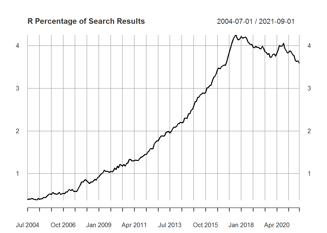
plot(tpl_xts$Python, main="Python Percentage of Search Results")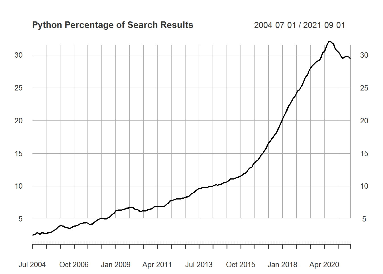
For both languages we can see a fairly strong rate of growth until recently. Notably, of the two languages, Python is considerably more popular. This may be due, in part, to its versatility for a wide variety of applications while R is more focused on statistical applications.
We now plot all of our data below.
plot(tpl_xts, main="Percentage of Search Results By Language")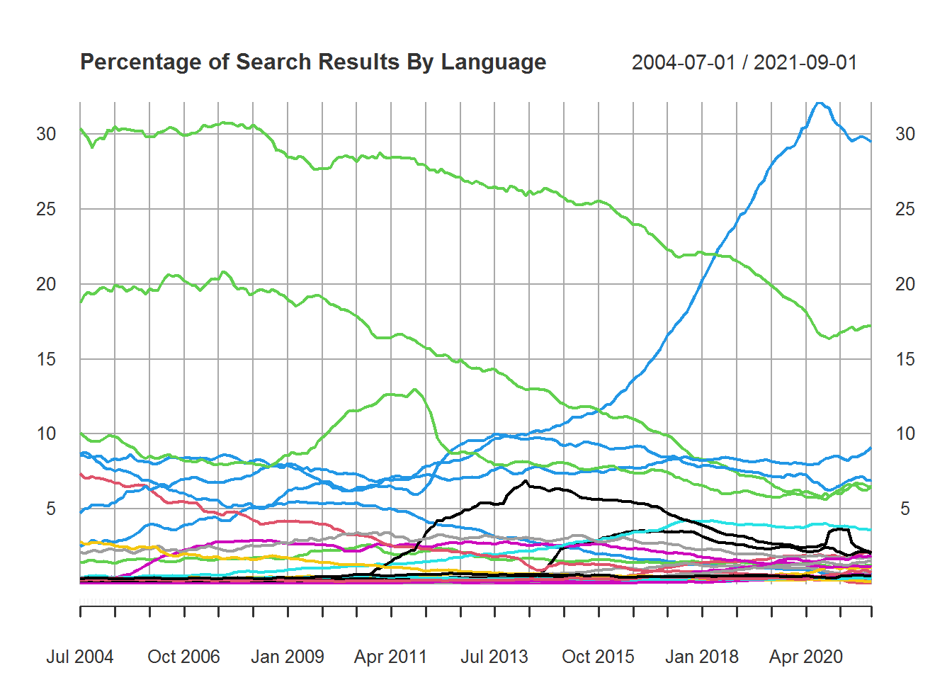
While the above plot doesn’t label any of the results and is fairly messy was can see a few interesting trends. Firstly, that Python has really broken away from the competition in the past few years to become the most searched programming language. Secondly, that during that same time a couple other popular languages have fallen in popularity. Visiting the PYPL website we can see that our current most searched languages are 1) Python, 2) Java, and 3) Javascript.
Conclusion
In this project we were able to show how we can manipulate strings in R in a variety of ways to get the results we need. We also saw how useful using the right tool for a job can be. With the strptime function we can manipulate date objects much quicker and for more formats of strings. Finally, we were able to see a bit of the most popular programming languages based on about 17 years of data.