Introduction
In this post we will explore two datasets on United States national parks. The first dataset will focus on the location and physical size of the parks. The second dataset will focus on the species living in the parks. Our source for these datasets can be found at Kaggle by following this link.
We will use many packages in this post. We have two primary types of packages: general use helper packages and spatial packages for geographical maps. We list our packages below:
library(dplyr)
library(magrittr)
library(here)
library(ggplot2)
library(tidyverse)

library(rworldmap)
library(rgeos)
library(sf)
library(ggspatial)
library(rnaturalearth)
library(rnaturalearthdata)

library(RColorBrewer)
Now that are packages are loaded we upload our datasets into the dataframes parks and species.
parks <- read.csv(here('csv', 'kaggle_national_parks', 'parks.csv'))
species <- read.csv(here('csv', 'kaggle_national_parks', 'species.csv'))
With our datasets loaded we will split our work into two sections. The first section will deal with the park dataset and uncovering some geographical data. The second section will take a closer look at the species that are present in the parks using the species dataset.
Section 1: Exploring General Park Data
Here we will look at the structure of the parks dataset and then manipulate the dataset to illustrate some interesting facts. In the structure of the data we see (below) that we have 56 national parks and they are being described by 6 variables.
str(parks)## 'data.frame': 56 obs. of 6 variables:
## $ Park.Code: chr "ACAD" "ARCH" "BADL" "BIBE" ...
## $ Park.Name: chr "Acadia National Park" "Arches National Park" "Badlands National Park" "Big Bend National Park" ...
## $ State : chr "ME" "UT" "SD" "TX" ...
## $ Acres : int 47390 76519 242756 801163 172924 32950 35835 337598 241904 46766 ...
## $ Latitude : num 44.4 38.7 43.8 29.2 25.6 ...
## $ Longitude: num -68.2 -109.6 -102.5 -103.2 -80.1 ...The first thing we would like to do with our dataset is determine which states have the most national parks. This question is not entirely trivial due to the fact that some national parks are in more than one state. Below we count the number of national parks in a state by allowing parks to be counted in each state they intersect with.
# Note that all state abbreviations are of length 2.
states <- NULL
for (value in parks$State) {
    if (nchar(value) > 2) {
        value <- strsplit(value, ', ')
        states <- c(states, unlist(value))}
    else {
        states <- c(states, value)}}
Our results are shown in the following table:
table(states) %>%
    as.data.frame() %>%
    arrange(desc(Freq))
## states Freq
## 1 AK 8
## 2 CA 8
## 3 UT 5
## 4 CO 4
## 5 AZ 3
## 6 FL 3
## 7 WA 3
## 8 HI 2
## 9 MT 2
## 10 NV 2
## 11 SD 2
## 12 TX 2
## 13 WY 2
## 14 AR 1
## 15 ID 1
## 16 KY 1
## 17 ME 1
## 18 MI 1
## 19 MN 1
## 20 NC 1
## 21 ND 1
## 22 NM 1
## 23 OH 1
## 24 OR 1
## 25 SC 1
## 26 TN 1
## 27 VA 1So far, we can see that Alaska and California are tied for having the most national parks; each with a count of 8. Let’s take a quick look at our data from a geographical perspective. Looking a map of North America we plot the location of each national park using their latitude and longitude. We get the following simple map below.
# get map
worldmap <- getMap(resolution = "coarse")
# plot world map
plot(worldmap, col = "lightgrey",
     border = "darkgray",
     xlim = c(-170, -60), ylim = c(20, 70),
     bg = "aliceblue", asp = 1,
     main = "United States National Parks Locations")

points(parks$Longitude, parks$Latitude, col = "red")
For a more sophisticated map we will follow some of the tricks found at this site. To begin with, for illustrative purposes, we show a map of the entire world.
# load data
world <- ne_countries(scale = "medium", returnclass = "sf")
# gene world map
ggplot(data = world) +
  geom_sf() +
  labs( x = "Longitude", y = "Latitude") +
  ggtitle("World map", subtitle = paste0("(", length(unique(world$admin)), " countries)"))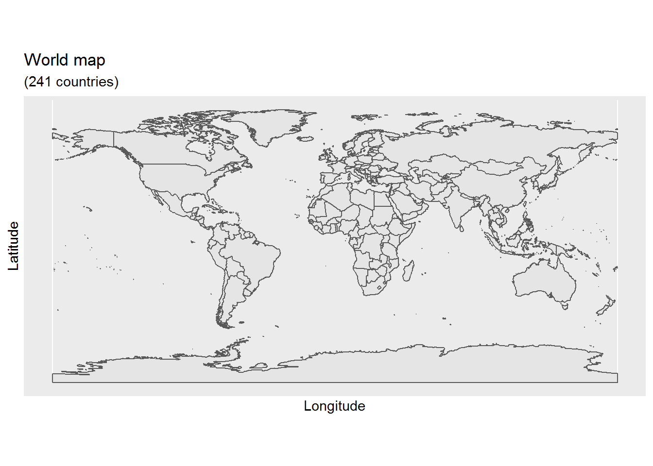
This is too zoomed out and so in our next chunk of code we restrict our location in the map to North America. We do this with the location of our national parks shown and using the number of acres in a park to illustrate the relative size of the park.
# gene world map
ggplot(data = world) +
  geom_sf() + ggtitle("United States National Parks Locations and Relative Sizes") +
  labs( x = "Longitude", y = "Latitude") +
  coord_sf(xlim = c(-170.00, -60.00), ylim = c(20.00, 70.00)) +
  annotation_scale(location = "br", width_hint = 0.5) +
  annotation_north_arrow(location = "br", which_north = "true",
                         pad_x = unit(0.75, "in"), pad_y = unit(0.5, "in"),
                         style = north_arrow_fancy_orienteering) +
  theme(panel.grid.major = element_line(color = "gray60", linetype = "dashed", size = 0.25),
         panel.background = element_rect(fill = "aliceblue")) +
  geom_point(data=parks, aes(x=Longitude, y=Latitude, size=Acres), color="red", alpha=0.5) +
  scale_size(range = c(1,12))
## Scale on map varies by more than 10%, scale bar may be inaccurate
Notice that in the above map our largest parks seem to primarily be in Alaska and that most of the national parks are in the Western half of the United States. To see both our largest and smallest parks we sort our parks below and then display the largest 6 and then smallest 6 parks.
sorted_parks <- parks[order(-parks$Acres), ]# largest parks
head(sorted_parks[ , 1:4])## Park.Code Park.Name State Acres
## 53 WRST Wrangell - St Elias National Park and Preserve AK 8323148
## 19 GAAR Gates Of The Arctic National Park and Preserve AK 7523898
## 16 DEVA Death Valley National Park CA, NV 4740912
## 33 KATM Katmai National Park and Preserve AK 3674530
## 15 DENA Denali National Park and Preserve AK 3372402
## 21 GLBA Glacier Bay National Park and Preserve AK 3224840# smallest parks
tail(sorted_parks[ , 1:4])## Park.Code Park.Name State Acres
## 14 CUVA Cuyahoga Valley National Park OH 32950
## 28 HALE Haleakala National Park HI 29094
## 52 WICA Wind Cave National Park SD 28295
## 44 PINN Pinnacles National Park CA 26606
## 12 CONG Congaree National Park SC 26546
## 30 HOSP Hot Springs National Park AR 5550This shows us that, asides from Death Valley National Park in California and Nevada, Alaska contains the largest national parks in the United States. Additionally, we can see that Hot Springs National Park is the smallest national park by a considerable margin.
Section 2: Exploring Park Species Data
We now begin our exploration of the species dataset by looking at its dataframe structure.
str(species)## 'data.frame': 119248 obs. of 14 variables:
## $ Species.ID : chr "ACAD-1000" "ACAD-1001" "ACAD-1002" "ACAD-1003" ...
## $ Park.Name : chr "Acadia National Park" "Acadia National Park" "Acadia National Park" "Acadia National Park" ...
## $ Category : chr "Mammal" "Mammal" "Mammal" "Mammal" ...
## $ Order : chr "Artiodactyla" "Artiodactyla" "Carnivora" "Carnivora" ...
## $ Family : chr "Cervidae" "Cervidae" "Canidae" "Canidae" ...
## $ Scientific.Name : chr "Alces alces" "Odocoileus virginianus" "Canis latrans" "Canis lupus" ...
## $ Common.Names : chr "Moose" "Northern White-Tailed Deer, Virginia Deer, White-Tailed Deer" "Coyote, Eastern Coyote" "Eastern Timber Wolf, Gray Wolf, Timber Wolf" ...
## $ Record.Status : chr "Approved" "Approved" "Approved" "Approved" ...
## $ Occurrence : chr "Present" "Present" "Present" "Not Confirmed" ...
## $ Nativeness : chr "Native" "Native" "Not Native" "Native" ...
## $ Abundance : chr "Rare" "Abundant" "Common" "" ...
## $ Seasonality : chr "Resident" "" "" "" ...
## $ Conservation.Status: chr "" "" "Species of Concern" "Endangered" ...
## $ X : chr "" "" "" "" ...We can see that this is a much larger dataset with 119248 observations and 14 variables. To keep things simple, we will only focus on a few of the variables. To ensure that a species is currently in the park and not just a historical sighting we focus on when the variable Occurrence is equal to the value Present.
species_present <- species[species$Occurrence == "Present", ]Below we calculate the percentage of data that we are removing from our dataset.
# data lost when filtering Occurrence for "Present"
1 - nrow(species_present) / nrow(species)
## [1] 0.3016403This shows us that we removed approximately 30% of our data. We now display our national parks in order of which parks have the most species. We can see below that the Great Smokey Mountains National Park has the most species.
species_present %>% count(Park.Name, sort=TRUE)## Park.Name n
## 1 Great Smoky Mountains National Park 3888
## 2 Yellowstone National Park 3481
## 3 North Cascades National Park 3029
## 4 Rocky Mountain National Park 2969
## 5 Hawaii Volcanoes National Park 2749
## 6 Shenandoah National Park 2631
## 7 Grand Canyon National Park 2565
## 8 Glacier National Park 2402
## 9 Congaree National Park 2097
## 10 Haleakala National Park 2088
## 11 Big Bend National Park 2011
## 12 Mammoth Cave National Park 1941
## 13 Yosemite National Park 1905
## 14 Channel Islands National Park 1847
## 15 Sequoia and Kings Canyon National Parks 1819
## 16 Grand Teton National Park 1801
## 17 Everglades National Park 1791
## 18 Cuyahoga Valley National Park 1787
## 19 Guadalupe Mountains National Park 1581
## 20 Saguaro National Park 1578
## 21 Redwood National Park 1537
## 22 Wrangell - St Elias National Park and Preserve 1511
## 23 Death Valley National Park 1471
## 24 Carlsbad Caverns National Park 1427
## 25 Mount Rainier National Park 1378
## 26 Olympic National Park 1367
## 27 Biscayne National Park 1330
## 28 Zion National Park 1317
## 29 Pinnacles National Park 1281
## 30 Glacier Bay National Park and Preserve 1250
## 31 Voyageurs National Park 1185
## 32 Acadia National Park 1172
## 33 Isle Royale National Park 1169
## 34 Capitol Reef National Park 1163
## 35 Crater Lake National Park 1123
## 36 Mesa Verde National Park 1112
## 37 Wind Cave National Park 1059
## 38 Lassen Volcanic National Park 1020
## 39 Denali National Park and Preserve 1002
## 40 Lake Clark National Park and Preserve 984
## 41 Great Basin National Park 967
## 42 Theodore Roosevelt National Park 931
## 43 Badlands National Park 909
## 44 Canyonlands National Park 866
## 45 Joshua Tree National Park 862
## 46 Great Sand Dunes National Park and Preserve 814
## 47 Katmai National Park and Preserve 799
## 48 Bryce Canyon National Park 790
## 49 Arches National Park 750
## 50 Dry Tortugas National Park 745
## 51 Petrified Forest National Park 734
## 52 Gates Of The Arctic National Park and Preserve 724
## 53 Black Canyon of the Gunnison National Park 689
## 54 Hot Springs National Park 680
## 55 Kenai Fjords National Park 645
## 56 Kobuk Valley National Park 555Let’s take a visual approach to seeing what type of species show up across the national parks. For this we create a bar plot with a pie chart added to show the relative proportions of the data. For a few good references we use https://www.statology.org/ggplot-pie-chart/ for our pie charts, we use r-bloggers for demonstrating extended color palettes, and to put our pie chart into our ggplot we use another article from r-bloggers. Let’s take a look at the result below:
species_categories <- as.data.frame(table(species_present$Category))
names(species_categories)[1] <- "Category"

color_count = nrow(species_categories)
get_palette = colorRampPalette(brewer.pal(9, "Set1"))

p1 <- ggplot(species_categories, aes(x="", y=Freq, fill=Category)) +
    geom_bar(stat="identity", width=1, show.legend=FALSE) +
    theme_void() +
    coord_polar("y", start=0) +
    labs(x = NULL, y = NULL, fill = NULL) +
    scale_fill_manual(values=get_palette(color_count))

p2 <- ggplot(species_categories, aes(x=reorder(Category, -Freq), y=Freq, fill=Category)) +
    geom_bar(stat="identity") +
    theme_minimal() + ggtitle("United States National Parks") +
    geom_text(aes(label = paste0(Freq, "")), size=3, position = position_stack(vjust=0.5), check_overlap = TRUE) +
    scale_fill_manual(values=get_palette(color_count)) + xlab("Category") + ylab("Count") +
    scale_x_discrete(breaks = NULL) +
    theme(axis.ticks.x = element_blank(), axis.text.x=element_blank())

p2 + annotation_custom(ggplotGrob(p1), xmin=3, xmax=14, ymin=5000, ymax=50000)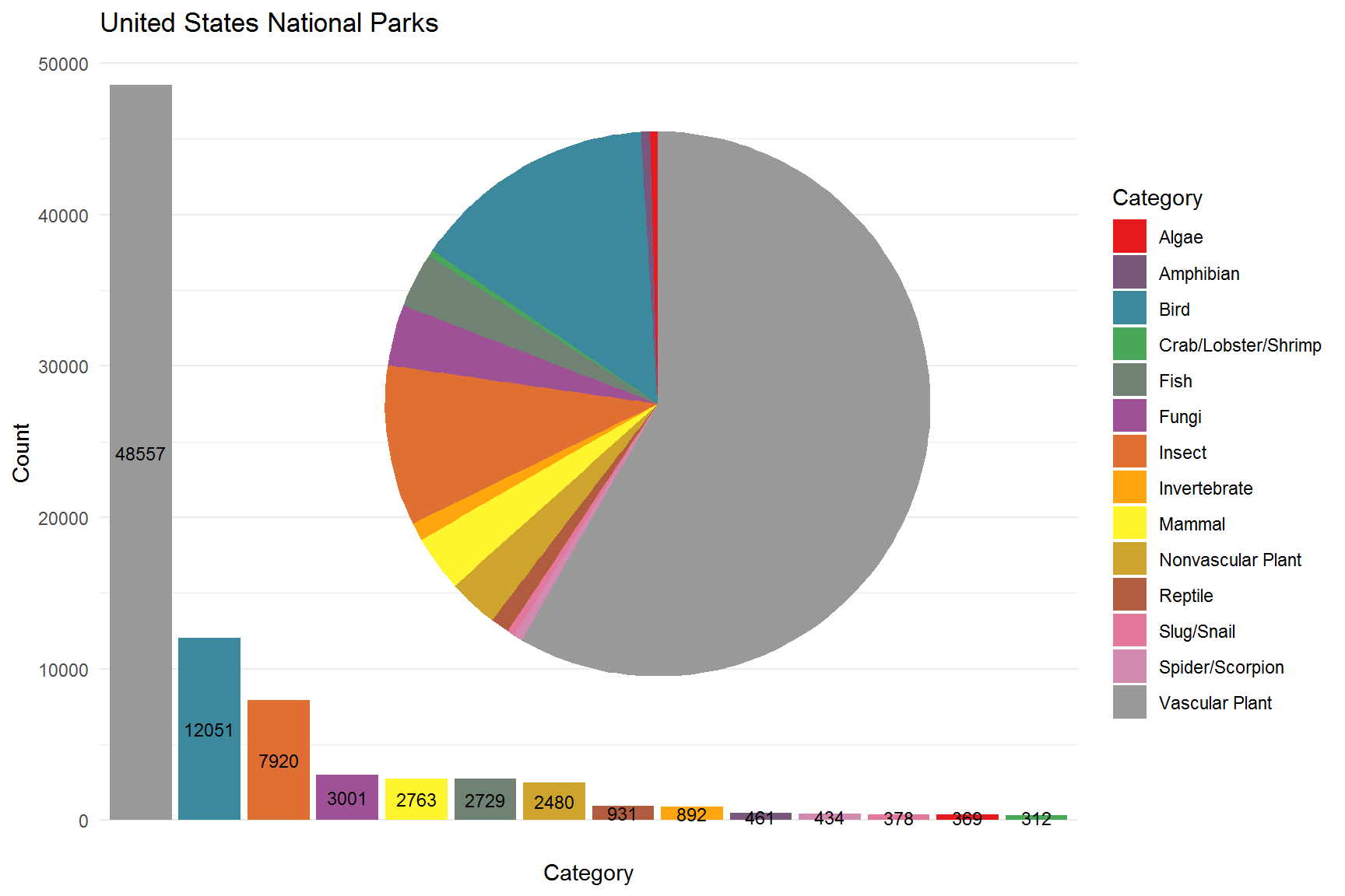
This shows that overall vascular plants are the most prevalent species. Behind this we have birds followed by insects. Since this is an overview of all of our parks, let’s take a closer look at two of our national parks to see if there is a different local story.
We first explore the Everglades National Park:

This park follows the overall pattern for the first two spots, but noticeably we have many more species classified as fish compared to the remaining groups. We also note that no insects among other species show up in this data. This is more likely to indicate this type of species was not counted as opposed to simply not being present. This also indicates that our overall numbers may be off.
Our second national park of interest will be Yellowstone National Park. We look at our species distribution below:
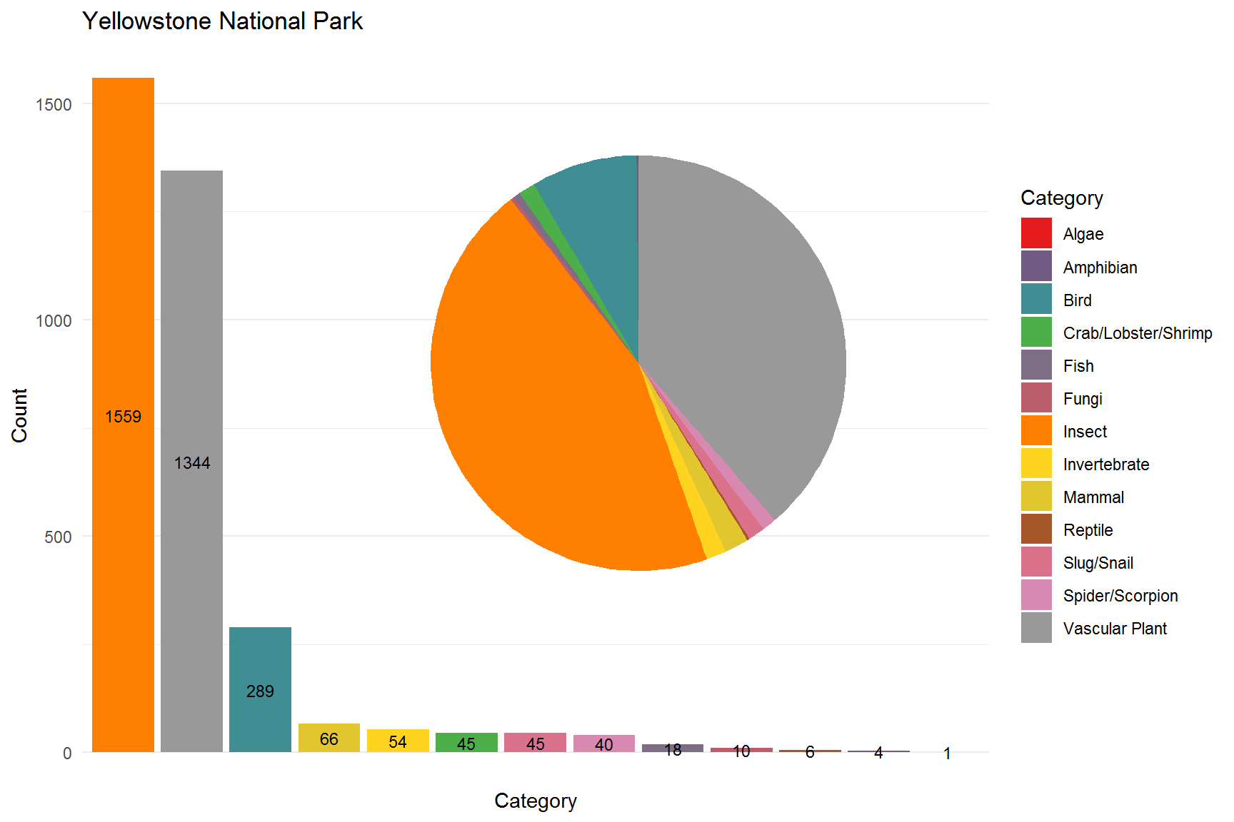
Here we can see that insects are the most prevalent species with vascular plants second and birds coming in third. Since this dataset includes all the common species we can be more confident in the overall results.
Conclusion
With our goal of data exploration we were able to uncover a few interesting details. The largest national parks are in Alaska. Most of the national parks are in the Western half of the United states. Plants are the most prevalent species over all the national parks. And perhaps most importantly we are reminded that even with a very large dataset, sometimes a simple logical check can show that data is missing which could otherwise go unnoticed. This demonstrates the complexity and importance of careful data cleaning in making good results. Unless of course there are actually no insects in the Everglades.