Principle Component Analysis (PCA) Face Reconstruction

Introduction

For this project we will be using PCA towards the goal of image compression and reconstruction. We use 27 of the 28 faces in the Extended Yale Face Database B. This dataset can be found at http://vision.ucsd.edu/~leekc/ExtYaleDatabase/ExtYaleB.html by clicking the “Original Images” link. This dataset has 9 poses for each person labeled 0 to 8. We omit one face due to the poses being labeled from 1 to 9. While the original dataset has 64 illumination conditions for each pose, we will only use the “+000E+00” default condition and stick with a smaller dataset with 9 images for each person’s face. From this, we split the data into a testing set with pose 0 for each individual and a training set with poses 1 through 8 for each individual.

We will be using the R libraries dplyr, magrittr, here, and pixmap for our analysis. After loading up our libraries we quickly run the code below to figure out the size of our dataset.

training_folder <- here::here("csv", "yaleBext_face_dataset", "train")
file_names <- list.files(training_folder)
n <- length(file_names)

We see that we have 216 images in the training set. Note that our images have the file extension .pgm or portable gray map. So each file is a grayscale image. We use the pixmap package to load our data into R.

Examining the Data

Using the read.pnm function from pixmap we load in our data.

image_list <- here::here("csv", "yaleBext_face_dataset", "train", file_names) %>%
    lapply(read.pnm, cellres=1)

Now that we have our training set in R, let’s take a look at the first element to see what we are working with.

str(image_list[[1]])

## Formal class 'pixmapGrey' [package "pixmap"] with 6 slots
##   ..@ grey    : num [1:480, 1:640] 0.78 0.757 0.749 0.745 0.714 ...
##   ..@ channels: chr "grey"
##   ..@ size    : int [1:2] 480 640
##   ..@ cellres : num [1:2] 1 1
##   ..@ bbox    : num [1:4] 0 0 640 480
##   ..@ bbcent  : logi FALSE

As we can see we are working with an object of class pixmapGrey with 6 slots. Of particular interest is the grey slot which holds a matrix with 480 rows and 640 columns. It contains values between 0 and 1 representing shades of gray. Blacker values are closer to 0 while whiter values are closer to 1. To take a look at the image we can call the plot function on the object:

plot(image_list[[1]])

As we can see, we have a persons face with a somewhat noisy background (not a single grayscale color). Cropping the face out from the rest of the image could be good for face recognition purposes, but is not strictly needed for our current exploratory purposes. So we will not be cropping the images.

Now that we’ve had a glimpse of our data we need to consider the next step. Since our goal is to apply PCA to help with image deconstruction and reconstruction we need to consider the size of our data. We have already established that our training set has 216 observations. For the number of covariates we need to know the total number of pixels.

size <- image_list[[1]]@size
p <- size[1] * size[2]

Our calculation shows that we have 307200 covariates to work with. So we will have a very wide dataset with 216 observations by 307200 covariates.

Finding the Average Face

We now begin combining our data into a matrix and then finding the so called average face for our images.

X <- matrix(0, n, p)  # initialize matrix of face pixels

for(i in 1:n){
    # store face pixels in matrix rows
    X[i, ] <- c(image_list[[i]]@grey)  # store face pixels in matrix
}

We now have a 216 by 307200 matrix with each row corresponding to a single image. From this we can calculate the average face as the average grayscale value for each pixel across all images. Notice the importance of having images of the same dimensions for this to work correctly.

# The average face
X_average <- colMeans(X)

Now that we have the average face as a vector we convert it to a matrix and then finally to a pixmapGrey object. Once we have our pixmap object we plot the average face to see what it looks like.

# setting things up to view the average face
average_matrix <- matrix(X_average, nrow=size[1], ncol=size[2])
average_face <- pixmapGrey(average_matrix, cellres=1)
plot(average_face)

From our plot it appears that the average face shows us roughly where peoples faces are in the picture and what the background is. Considering the first image we looked at along with the double images of the background it appears that the camera did not stay entirely in the same position.

Finding Eigenfaces

Now that we have the average face we need to find eigenvalues and eigenvectors from the covariance matrix for our observations. Doing this directly would be computationally expensive due to the large number of covariates. Indeed, a direct computation would require creating a covariance matrix of size 307200 by 307200 and then trying to compute the eigenvalues and eigenvectors. Fortunately, we have a better method which allows us to find the eigenvalues and eigenvectors using a 216 by 216 matrix based on the observation size. We go through the steps below, but will not touch on the theory except to mention it pertains to matrix rank. Note that all our matrix values are between 0 and 1 and do not need to be rescaled. Additionally, we will use the average face to center our data.

# Initialize matrix W of pixels centered by the grayscale
W <- matrix(0, p, n)

# Fill in W
for(i in 1:n){
    W[, i] <- X[i, ] - X_average
}

# Since we have more covariates than observations we use
B <- t(W) %*% W
# We then find the eigenpairs for B instead of from the
# covariance matrix of W (which would be huge)
eigen_results <- eigen(B, only.values=F)
sum_eigs <- sum(diag(B))

# Expected Loss of Information
ELOI <- array(0,n)

Below we print out the Expected Loss of Information (ELOI) for number of eigenvectors kept corresponding to the largest eigenvalues being kept.

#calculated Expected Loss of Information (ELOI)
for(k in 1:n){
    ELOI[k] <- 1 - sum(eigen_results$values[1:k]) / sum_eigs
    print(paste(k, " ", ELOI[k], sep=""))
}

## [1] "1 0.831094794555602"
## [1] "2 0.676263290756113"
## [1] "3 0.57092835234447"
## [1] "4 0.500450167462506"
## [1] "5 0.450197365972926"
## [1] "6 0.408839349539243"
## [1] "7 0.374639520538796"
## [1] "8 0.34348261453641"
## [1] "9 0.319059612795088"
## [1] "10 0.296864679393487"
## [1] "11 0.276446188120384"
## [1] "12 0.261093643925808"
## [1] "13 0.246603761013929"
## [1] "14 0.233269841138626"
## [1] "15 0.220964892462174"
## [1] "16 0.209515237253156"
## [1] "17 0.199911022904271"
## [1] "18 0.19071919720734"
## [1] "19 0.182522131395531"
## [1] "20 0.175203557642719"
## [1] "21 0.168834606214963"
## [1] "22 0.162810561916729"
## [1] "23 0.157011603613169"
## [1] "24 0.151894260534421"
## [1] "25 0.147140880575706"
## [1] "26 0.142541546911696"
## [1] "27 0.138157042147818"
## [1] "28 0.134177376219966"
## [1] "29 0.130387512992454"
## [1] "30 0.126790026238458"
## [1] "31 0.123258988322238"
## [1] "32 0.120131574854443"
## [1] "33 0.117109660290326"
## [1] "34 0.114266182291172"
## [1] "35 0.111477840270979"
## [1] "36 0.108865744441815"
## [1] "37 0.106380068024622"
## [1] "38 0.103994662854637"
## [1] "39 0.101641209115275"
## [1] "40 0.099376458274136"
## [1] "41 0.0971939933309057"
## [1] "42 0.0950421454112894"
## [1] "43 0.0929819230929866"
## [1] "44 0.0909425703366573"
## [1] "45 0.0889609540279038"
## [1] "46 0.0870780350202423"
## [1] "47 0.0852813805381858"
## [1] "48 0.0835068072904699"
## [1] "49 0.0817575673861302"
## [1] "50 0.08003825845492"
## [1] "51 0.0784367297663275"
## [1] "52 0.0768733523176452"
## [1] "53 0.075383047049053"
## [1] "54 0.0739072849539137"
## [1] "55 0.0724797146523648"
## [1] "56 0.0710920645107931"
## [1] "57 0.0697507023833395"
## [1] "58 0.0684438389995961"
## [1] "59 0.0671876064895151"
## [1] "60 0.0659518074612522"
## [1] "61 0.0647488890573066"
## [1] "62 0.0635758875665632"
## [1] "63 0.0624357267132368"
## [1] "64 0.0613027601990275"
## [1] "65 0.0601912804240219"
## [1] "66 0.0591042111613344"
## [1] "67 0.0580506555404717"
## [1] "68 0.0570183762743385"
## [1] "69 0.0560121544790192"
## [1] "70 0.0550145761751555"
## [1] "71 0.0540536358094151"
## [1] "72 0.0531265435560463"
## [1] "73 0.052207281603603"
## [1] "74 0.0512948700157249"
## [1] "75 0.0504014844474098"
## [1] "76 0.0495259677035542"
## [1] "77 0.0486608274218302"
## [1] "78 0.0478190831350263"
## [1] "79 0.0469872347669856"
## [1] "80 0.0461607446144598"
## [1] "81 0.0453780963513345"
## [1] "82 0.0446014739529774"
## [1] "83 0.0438384391653882"
## [1] "84 0.0430811991580813"
## [1] "85 0.0423283711331384"
## [1] "86 0.041588908889348"
## [1] "87 0.0408637142133537"
## [1] "88 0.0401447507626159"
## [1] "89 0.0394335761687518"
## [1] "90 0.0387499385515021"
## [1] "91 0.0380692567726145"
## [1] "92 0.037410093726652"
## [1] "93 0.0367598984209337"
## [1] "94 0.0361166698742973"
## [1] "95 0.0354784192486991"
## [1] "96 0.0348538166018603"
## [1] "97 0.0342519527263904"
## [1] "98 0.0336549218494731"
## [1] "99 0.0330630699057519"
## [1] "100 0.0324762087344314"
## [1] "101 0.0319048432351258"
## [1] "102 0.0313391194019947"
## [1] "103 0.0307880005048352"
## [1] "104 0.0302449104979967"
## [1] "105 0.0297070693701803"
## [1] "106 0.0291751259028917"
## [1] "107 0.0286590853227198"
## [1] "108 0.0281502424663673"
## [1] "109 0.0276498358975289"
## [1] "110 0.0271577319897847"
## [1] "111 0.0266708480059737"
## [1] "112 0.0261921984632471"
## [1] "113 0.0257217955933567"
## [1] "114 0.0252616865600112"
## [1] "115 0.024805739348882"
## [1] "116 0.0243583683018972"
## [1] "117 0.0239138440434182"
## [1] "118 0.023475059595892"
## [1] "119 0.0230397287220004"
## [1] "120 0.0226114946305011"
## [1] "121 0.0221899477929612"
## [1] "122 0.021774660139845"
## [1] "123 0.0213617210892491"
## [1] "124 0.0209518892810432"
## [1] "125 0.0205585114494022"
## [1] "126 0.0201678137477275"
## [1] "127 0.0197808383626159"
## [1] "128 0.0193999755618246"
## [1] "129 0.0190198599615383"
## [1] "130 0.018644699296159"
## [1] "131 0.0182763529885501"
## [1] "132 0.017912083292962"
## [1] "133 0.0175554696926032"
## [1] "134 0.0172008017358802"
## [1] "135 0.0168507591129911"
## [1] "136 0.0165028948029071"
## [1] "137 0.0161627128278672"
## [1] "138 0.0158229916040238"
## [1] "139 0.0154882619565467"
## [1] "140 0.0151564790330365"
## [1] "141 0.0148284248736709"
## [1] "142 0.0145032801230339"
## [1] "143 0.0141862409208432"
## [1] "144 0.0138698254171475"
## [1] "145 0.0135599400543888"
## [1] "146 0.0132569809841638"
## [1] "147 0.0129551855555085"
## [1] "148 0.0126612972214829"
## [1] "149 0.0123705571625934"
## [1] "150 0.0120836825155033"
## [1] "151 0.0118001404289657"
## [1] "152 0.011521655066936"
## [1] "153 0.0112459866631937"
## [1] "154 0.0109773844664582"
## [1] "155 0.010711302636609"
## [1] "156 0.0104503534040455"
## [1] "157 0.0101925877454596"
## [1] "158 0.00994029170467881"
## [1] "159 0.00968937040141737"
## [1] "160 0.00944018252809042"
## [1] "161 0.00919404697241077"
## [1] "162 0.00895072774589201"
## [1] "163 0.008712218441701"
## [1] "164 0.00847531672560953"
## [1] "165 0.0082431747396815"
## [1] "166 0.00801391657063932"
## [1] "167 0.0077872701483741"
## [1] "168 0.00756213254914806"
## [1] "169 0.00733915937152751"
## [1] "170 0.00711891458956271"
## [1] "171 0.00690104146193893"
## [1] "172 0.00668636303893178"
## [1] "173 0.00647663277754162"
## [1] "174 0.00627011702460234"
## [1] "175 0.00606713747581666"
## [1] "176 0.00586470949067019"
## [1] "177 0.00566717885444867"
## [1] "178 0.00547023884760411"
## [1] "179 0.00527457208495097"
## [1] "180 0.0050837454820879"
## [1] "181 0.00489545324398344"
## [1] "182 0.00470913475629986"
## [1] "183 0.00452316146615572"
## [1] "184 0.00434327239682653"
## [1] "185 0.00416409182920063"
## [1] "186 0.00398759110580216"
## [1] "187 0.00381266696378069"
## [1] "188 0.00363942415424168"
## [1] "189 0.00347049442578529"
## [1] "190 0.00330332076232553"
## [1] "191 0.0031394285188987"
## [1] "192 0.00297878830634091"
## [1] "193 0.00281975285816161"
## [1] "194 0.00266219815304336"
## [1] "195 0.00250728695661051"
## [1] "196 0.0023559484126664"
## [1] "197 0.00220588736783545"
## [1] "198 0.00206047942902776"
## [1] "199 0.00191602501687338"
## [1] "200 0.00177458430773292"
## [1] "201 0.00163437531360167"
## [1] "202 0.00149439278845387"
## [1] "203 0.00135836113704391"
## [1] "204 0.00122688512948999"
## [1] "205 0.00109843412965349"
## [1] "206 0.000973294464933327"
## [1] "207 0.000853064454544139"
## [1] "208 0.000733992673184081"
## [1] "209 0.000619664948466436"
## [1] "210 0.000506145661771984"
## [1] "211 0.000395478813378314"
## [1] "212 0.000289928018979979"
## [1] "213 0.000185015764051277"
## [1] "214 8.44951118696979e-05"
## [1] "215 -4.44089209850063e-16"
## [1] "216 6.66133814775094e-16"

In order to compare the results, we will examine what happens with various levels of ELOI. Let’s start with having ELOI not more than 25%. This corresponds to keeping 13 eigenvectors.

# Based on ELOI we choose k = 13
collect_eigenvectors = function(k){
    eigen_kvalues <- eigen_results$values[1:k]
    eigen_kvectors <- eigen_results$vectors[,1:k]
    eigvec_Sigma_hat_k <- matrix(0, p, k)
    
    for(i in 1:k){
      eigvec_Sigma_hat_k[,i] <- c(1/sqrt(eigen_kvalues[i])) * (W %*% matrix(eigen_kvectors[, i], ncol = 1))
    }
    
    return(t(eigvec_Sigma_hat_k))
}


# Matrix of transposed eigenvectors
A_k <- collect_eigenvectors(k=13)

Since we are keeping 13 eigenvectors we could examine any of the corresponding eigenfaces. In this case we will look at the second eigenface.

# setting things up to view the second eigenface
eigenface_matrix <- matrix(A_k[2, ], nrow=size[1], ncol=size[2], byrow=F)
second_eigenface <- pixmapGrey(eigenface_matrix, cellres=1)

We plot the second eigenface below.

plot(second_eigenface)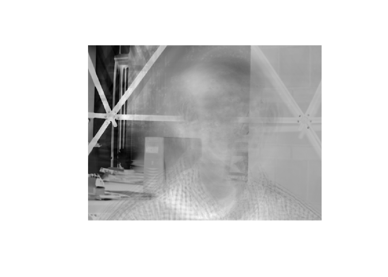

Face reconstruction

Using the 13 eigenfaces we just found, based on our choice of ELOI, let’s try to reconstruct a face. Using face 12 we will show the original face, deconstruct it by finding the PC representation and then reconstruct the image. We plot the original face below.

new_filepath = here::here("csv", "yaleBext_face_dataset", "test", "yaleB12_P00A+000E+00.pgm")
new_image <- read.pnm(new_filepath, cellres=1)
plot(new_image)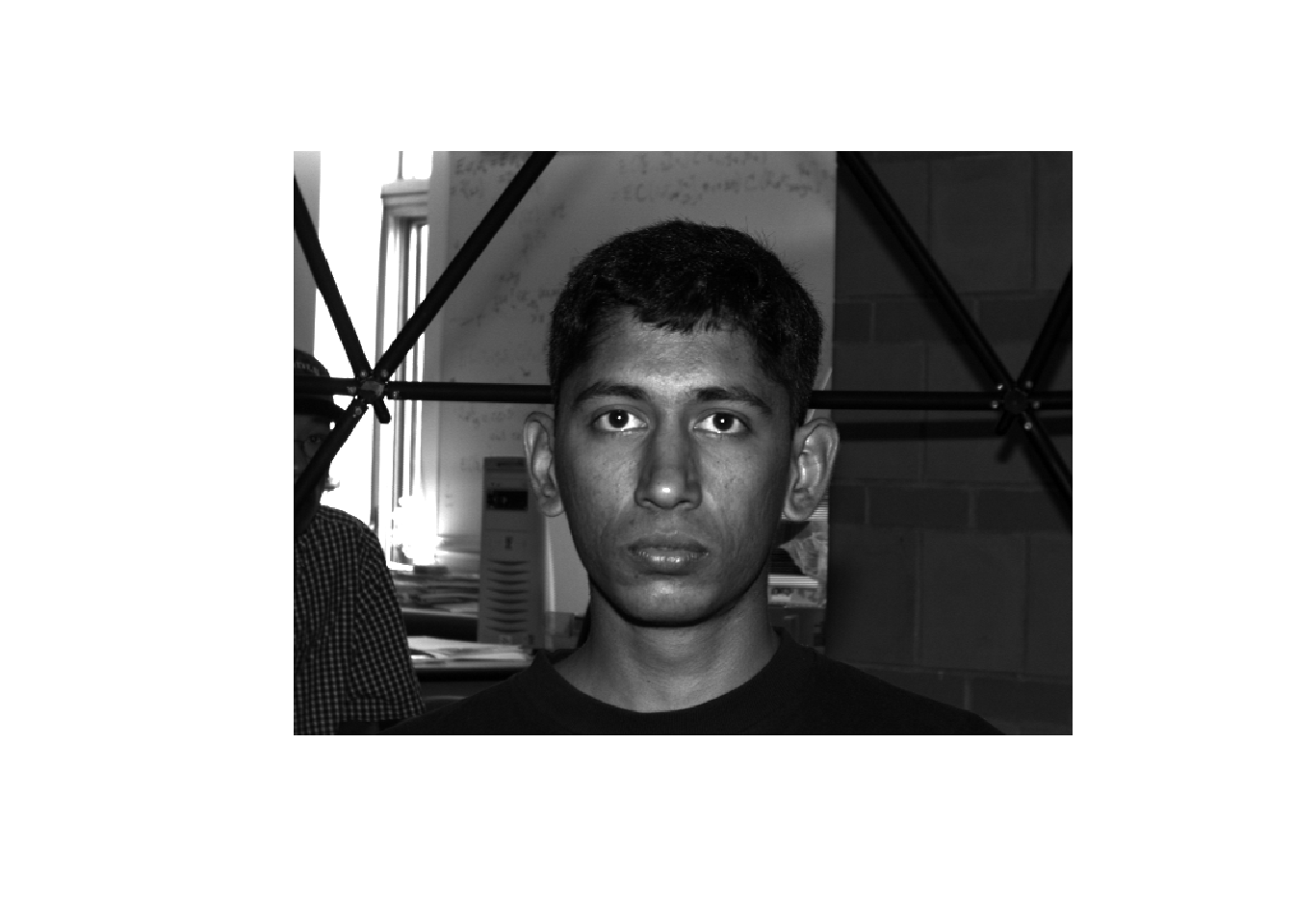

With this new image we deconstruct it using our PC representation. We then plot the face

# Reconstruct test image 12 from PCA
# To do this we create a function to deconstruct
# and then reconstruct the image
de_re_construct_face <- function(image, k){
    # PC representation for test image
    A_k <- collect_eigenvectors(k=k)
    PC_representation <- A_k %*%(matrix(c(image@grey) - X_average, ncol = 1))
    # Reconstruction of test image using PC representation
    reconstructed_observations <- X_average + t(A_k) %*% matrix(PC_representation, ncol = 1)
    reconstructed_image12_matrix <- matrix(reconstructed_observations, ncol=size[2])
    
    return(pixmapGrey(reconstructed_image12_matrix, cellres=1))
}


reconstructed_image12 <- de_re_construct_face(new_image, k=13)
plot(reconstructed_image12, xlab = "Reconstructed test image with k = 13 eigenfaces")

From this we can see that our images did a good job reconstructing the room, but not the face which is more variable throughout the images. Since our main interest is the faces this is a little disappointing. Other points of interest are that the person to the left of the screen does not show up and the dark hair from image 12 shows up a little bit along with a bit of the black shirt.

Repeated Face Reconstruction

Now that we have things set up for image reconstruction we will repeat this process with lower and lower ELOI. With ELOI of at most 10 which corresponds to 40 eigenvectors we plot our result below.

reconstructed_image12 <- de_re_construct_face(new_image, k=40)
plot(reconstructed_image12, xlab = "Reconstructed test image with k = 40 eigenfaces")

This begins to show the eyes, though we see a pair of double eyes. We also see the person in the background start to show up. We try again with ELOI of 5 which corresponds to 76 eigenvectors.

reconstructed_image12 <- de_re_construct_face(new_image, k=76)
plot(reconstructed_image12, xlab = "Reconstructed test image with k = 76 eigenfaces")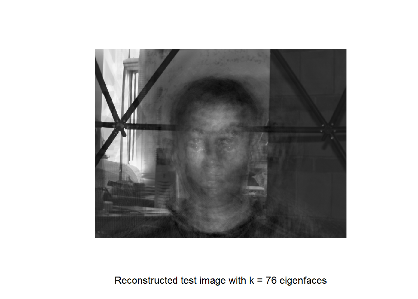

This does not seem significantly better. We now try with ELOI of at most 1 which corresponds to 158 eigenvectors.

reconstructed_image12 <- de_re_construct_face(new_image, k=158)
plot(reconstructed_image12, xlab = "Reconstructed test image with k = 158 eigenfaces")

In this case we are starting to clean up some of the noise. In particular it seems closer to having just a single pair of eyes. Finishing up with 215 eigenvectors we get the following.

reconstructed_image12 <- de_re_construct_face(new_image, k=215)
plot(reconstructed_image12, xlab = "Reconstructed test image with k = 215 eigenfaces")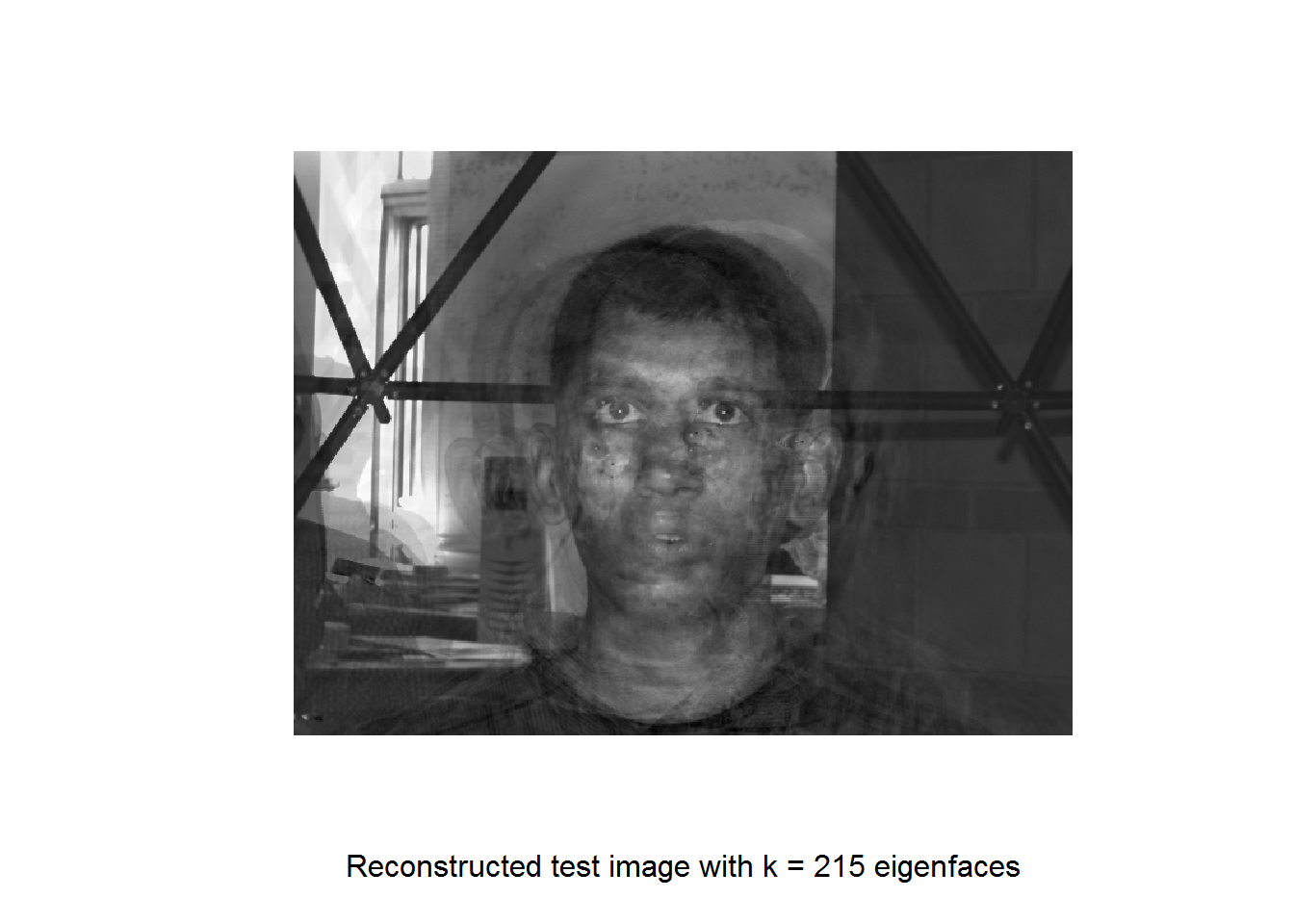

As we can see in this last image, the detail is enough to distinguish the individual from other individuals. Still, we cannot completely avoid noise. This is not surprising since we did not have the 307200 observations to compare with the number of pixels or covariates to be able to completely restore the image. This was not the goal either since otherwise we would have no interest in reducing the information in the image and could simply retain the original image. Nevertheless, to be able to restore the image to this degree using approximately 0.07% of the original variables represents a significant savings in terms of data storage space. Moreover, to reconstruct the images in this manner perfectly would require a matrix of size 307200 by 307200 which would be exceedingly large and likely impossible for most machines to compute with.

Restoring Additional faces

Before we wrap things up let’s try restoring a few other test faces for comparison.

new_filepath = here::here("csv", "yaleBext_face_dataset", "test", "yaleB26_P00A+000E+00.pgm")
new_image <- read.pnm(new_filepath, cellres=1)
reconstructed_image26 <- de_re_construct_face(new_image, k=215)

par(mfrow=c(1,2))
plot(new_image, main = "Original")
plot(reconstructed_image26, main = "Reconstructed")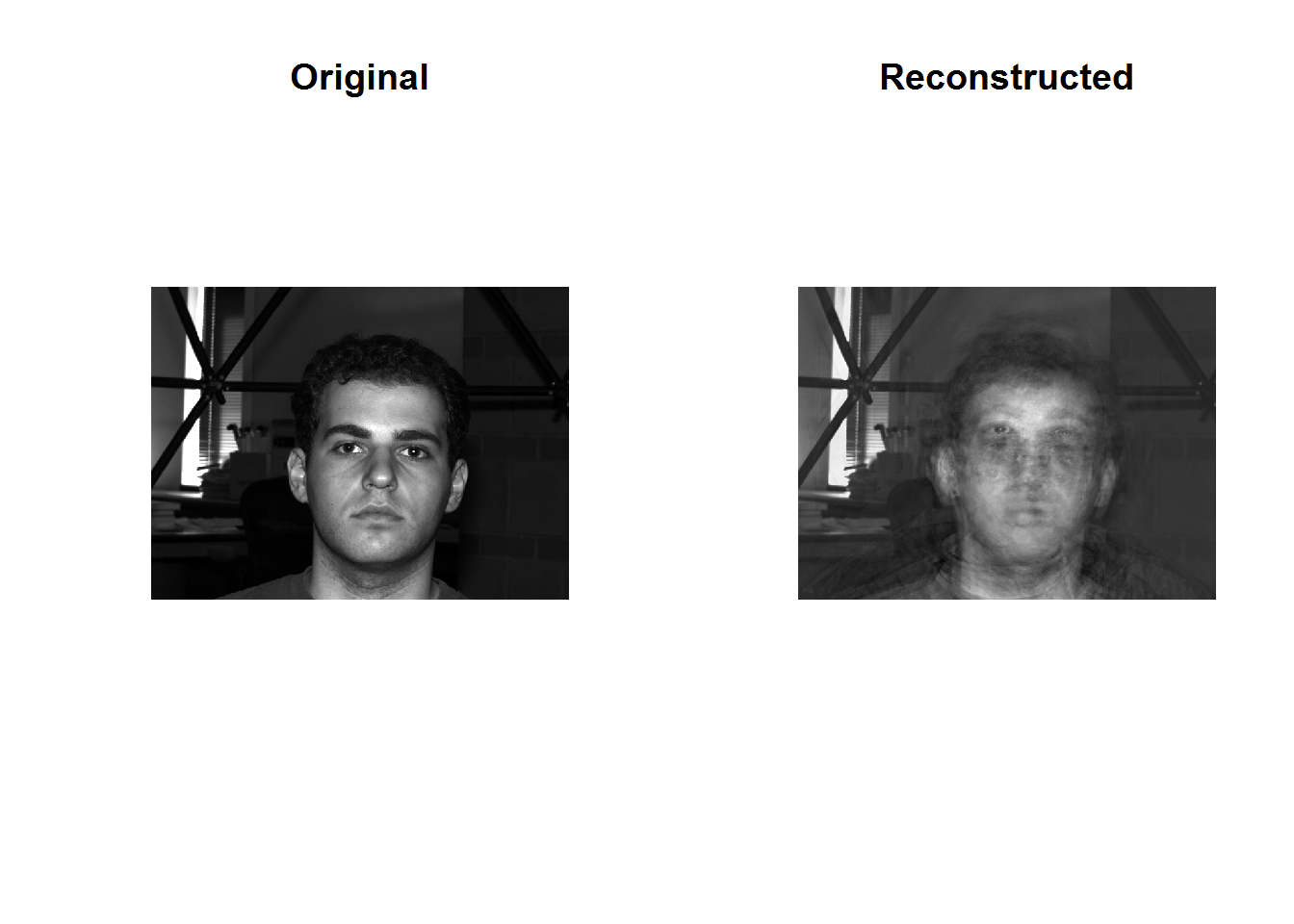

new_filepath = here::here("csv", "yaleBext_face_dataset", "test", "yaleB15_P00A+000E+00.pgm")
new_image <- read.pnm(new_filepath, cellres=1)
reconstructed_image15 <- de_re_construct_face(new_image, k=215)

par(mfrow=c(1,2))
plot(new_image, main = "Original")
plot(reconstructed_image15, main = "Reconstructed")

new_filepath = here::here("csv", "yaleBext_face_dataset", "test", "yaleB25_P00A+000E+00.pgm")
new_image <- read.pnm(new_filepath, cellres=1)
reconstructed_image25 <- de_re_construct_face(new_image, k=215)

par(mfrow=c(1,2))
plot(new_image, main = "Original")
plot(reconstructed_image25, main = "Reconstructed")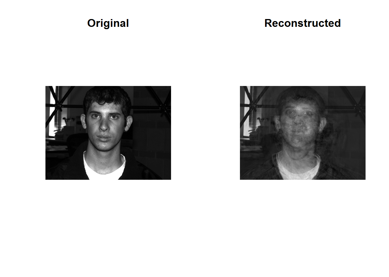

Conclusion

As we have seen, our PC representation of test images does not restore the images completely even with very low Expected Loss of Information (ELOI). This is not surprising since this value is based on the training images. Indeed, if we deconstruct and then reconstruct one of our training images we will see our images restored in alignment with the ELOI. If we want to be able to restore our test images to a higher degree we need to train our model with more images. Alternatively, if we only care about reconstruction of the face we could use a cropped version of the image of just the face. Then the model will not waste resources on trying to represent the environment.

Ultimately PCA is a very powerful technique for dimension reduction. Indeed, using only 0.07% of our original number of covariates we can roughly distinguish between the people. Moreover, if we want more power we can increase the sample size and if we want more precision we can use software to isolate the face. From here we could look into using these techniques for face recognition software. For example, we may be able to use software to check surveillance footage for a face from our database or alternatively check our database for a face or other biometric data. While PCA or other dimension reduction techniques may not be required they can likely speed up the computations while searching for a good match.