Introduction
For this project we will be looking more deeply at the 2011 India Census Data. To do this we will examine our data structure, utilize an additional dataset to help us visualize the data, and utilize some readily available information from the internet.
Once again we use the 2011 India Census data from Kaggle. To visualize our data we need some type of structure for the various regions in India. To this end we obtain data from https://gadm.org/download_country_v3.html and put India into the Country box. This gives us access to various levels of data in a variety of data types. For our purpose we will use the “R (sp)” data and focus on level 1 which corresponds to the regions of India. Note that sp refers to the sp package which deals with spatial data including points, lines, polygons and grids. This data will allow us to draw the lines for the regions in India.
Regions of India
In our 2011 India census data we have 35 distinct regions, however, we should have 36. In particular, our census data does not include information about Telangana. This means that without finding additional information or a more complete set of data we are unable to make accurate aggregations for the whole of India. So we will instead focus solely on aggregations for the 35 Regions we do have data for using the data from the 640 districts included in our census dataset.
Note that, when we refer to 36 regions we are actually referring to 28 States and 8 Union Territories. This is the case at least in early 2021. Note as well that some regions are very small geographically and are essentially cities. For example see the Union Territory of Puducherry. So considering things like population density could be interesting if you wanted to collect data on the area of each region.
Section 1: Set-up
Now that we have some context, we begin as always by loading up our packages.
library(sp)
library(here)
library(dplyr)
library(tmap)
library(tools)
library(stringr)
With our packages ready we next load up our data. This includes our census data as well as the geographical data needed to make our graphs.
geo_data <- here("csv", "kaggle_2020_dec_project",
                 "gadm36_IND_1_sp.rds") %>%
    readRDS()

india_census_data <- here("csv", "kaggle_2020_dec_project",
                          "india-districts-census-2011.csv") %>%
    read.csv()
Section 2: Exploring our Data Structures
As part of using a dataset we want to explore the structure and figure out what kind of data we are working with.
To begin with we look at the new geographical data. We do this using the str function and examine the first two layers.
str(geo_data, 2)## Formal class 'SpatialPolygonsDataFrame' [package "sp"] with 5 slots
## ..@ data :'data.frame': 36 obs. of 10 variables:
## ..@ polygons :List of 36
## ..@ plotOrder : int [1:36] 29 19 20 34 11 16 2 26 7 31 ...
## ..@ bbox : num [1:2, 1:2] 68.19 6.75 97.42 35.5
## .. ..- attr(*, "dimnames")=List of 2
## ..@ proj4string:Formal class 'CRS' [package "sp"] with 1 slotFrom this we can see that we are working with SpatialPolygonsDataFrame from the sp package. We also have data and a few more types of information relating to the geographical location and boundaries of India. Taking a closer look at the data.frame stored in the data variable and limiting our results for clarity we have:
geo_data@data[1:4, c("NAME_0", "NAME_1", "ENGTYPE_1")]## NAME_0 NAME_1 ENGTYPE_1
## 1 India Andaman and Nicobar Union Territory
## 12 India Andhra Pradesh State
## 23 India Arunachal Pradesh State
## 31 India Assam StateSo this data.frame includes the country name, region name, and whether the region is considered a State or a Union Territory. Moving on to our 2011 census data we look at the basic structure of our data.
str(india_census_data, 0)## 'data.frame': 640 obs. of 118 variables:We see that we are working directly with a data.frame with 640 observations, corresponding to districts, and 118 variables. To get a closer look at the variables we use the glimpse function from the dplyr package to see basic information about all 118 variables.
# We truncate long variable names for readability.
india_census_double <- india_census_data
names(india_census_double) <-
    str_trunc(names(india_census_double), 40)
glimpse(india_census_double)
## Rows: 640
## Columns: 118
## $ District.code <int> 1, 2, 3, 4, 5, 6, 7, 8, 9,...
## $ State.name <chr> "JAMMU AND KASHMIR", "JAMM...
## $ District.name <chr> "Kupwara", "Badgam", "Leh(...
## $ Population <int> 870354, 753745, 133487, 14...
## $ Male <int> 474190, 398041, 78971, 777...
## $ Female <int> 396164, 355704, 54516, 630...
## $ Literate <int> 439654, 335649, 93770, 862...
## $ Male_Literate <int> 282823, 207741, 62834, 563...
## $ Female_Literate <int> 156831, 127908, 30936, 299...
## $ SC <int> 1048, 368, 488, 18, 556, 4...
## $ Male_SC <int> 1046, 343, 444, 12, 406, 2...
## $ Female_SC <int> 2, 25, 44, 6, 150, 22987, ...
## $ ST <int> 70352, 23912, 95857, 12233...
## $ Male_ST <int> 36913, 12383, 47543, 62652...
## $ Female_ST <int> 33439, 11529, 48314, 59684...
## $ Workers <int> 229064, 214866, 75079, 518...
## $ Male_Workers <int> 190899, 162578, 53265, 398...
## $ Female_Workers <int> 38165, 52288, 21814, 12034...
## $ Main_Workers <int> 123837, 132003, 57125, 289...
## $ Marginal_Workers <int> 105227, 82863, 17954, 2293...
## $ Non_Workers <int> 641290, 538879, 58408, 889...
## $ Cultivator_Workers <int> 34680, 55299, 20869, 8266,...
## $ Agricultural_Workers <int> 56759, 36630, 1645, 3763, ...
## $ Household_Workers <int> 7946, 29102, 1020, 1222, 3...
## $ Other_Workers <int> 129679, 93835, 51545, 3862...
## $ Hindus <int> 37128, 10110, 22882, 10341...
## $ Muslims <int> 823286, 736054, 19057, 108...
## $ Christians <int> 1700, 1489, 658, 604, 958,...
## $ Sikhs <int> 5600, 5559, 1092, 1171, 11...
## $ Buddhists <int> 66, 47, 88635, 20126, 83, ...
## $ Jains <int> 39, 6, 103, 28, 10, 26, 16...
## $ Others_Religions <int> 13, 2, 54, 4, 2, 3, 2, 7, ...
## $ Religion_Not_Stated <int> 2522, 478, 1006, 289, 711,...
## $ LPG_or_PNG_Households <int> 15828, 15118, 13645, 3285,...
## $ Housholds_with_Electric_Lighting <int> 83071, 90190, 17250, 15824...
## $ Households_with_Internet <int> 762, 1999, 574, 235, 346, ...
## $ Households_with_Computer <int> 5256, 5892, 2150, 1005, 33...
## $ Rural_Households <int> 158438, 160649, 36920, 403...
## $ Urban_Households <int> 23226, 27190, 17474, 7774,...
## $ Households <int> 181664, 187839, 54394, 481...
## $ Below_Primary_Education <int> 60616, 68336, 10452, 12732...
## $ Primary_Education <int> 101642, 80862, 15181, 1908...
## $ Middle_Education <int> 99947, 83141, 17900, 20874...
## $ Secondary_Education <int> 74948, 66459, 16265, 16938...
## $ Higher_Education <int> 39709, 41367, 8923, 9826, ...
## $ Graduate_Education <int> 21751, 27950, 6197, 3077, ...
## $ Other_Education <int> 6402, 6857, 575, 408, 1884...
## $ Literate_Education <int> 405015, 374972, 75493, 829...
## $ Illiterate_Education <int> 289765, 342646, 32637, 398...
## $ Total_Education <int> 694780, 717618, 108130, 12...
## $ Age_Group_0_29 <int> 600759, 503223, 70703, 875...
## $ Age_Group_30_49 <int> 178435, 160933, 41515, 355...
## $ Age_Group_50 <int> 89679, 88978, 21019, 17488...
## $ Age.not.stated <int> 1481, 611, 250, 221, 704, ...
## $ Households_with_Bicycle <int> 3019, 10013, 609, 488, 846...
## $ Households_with_Car_Jeep_Van <int> 2988, 5091, 4271, 1847, 17...
## $ Households_with_Radio_Transistor <int> 59480, 66814, 15210, 10895...
## $ Households_with_Scooter_Motorcycle_Moped <int> 1808, 5848, 1289, 652, 240...
## $ Households_with_Telephone_Mobile_Phon... <int> 1445, 2509, 2646, 899, 190...
## $ Households_with_Telephone_Mobile_Phon... <int> 53437, 65783, 6331, 7733, ...
## $ Households_with_TV_Computer_Laptop_Te... <int> 495, 1655, 971, 249, 276, ...
## $ Households_with_Television <int> 26828, 54170, 13597, 8008,...
## $ Households_with_Telephone_Mobile_Phone <int> 56495, 72197, 13836, 10562...
## $ Households_with_Telephone_Mobile_Phon... <int> 1613, 3905, 4859, 1930, 26...
## $ Condition_of_occupied_census_houses_D... <int> 8463, 3733, 371, 575, 2047...
## $ Households_with_separate_kitchen_Cook... <int> 104172, 88806, 20134, 1775...
## $ Having_bathing_facility_Total_Households <int> 66361, 83385, 10304, 11887...
## $ Having_latrine_facility_within_the_pr... <int> 54335, 83615, 18780, 17649...
## $ Ownership_Owned_Households <int> 104807, 98036, 19387, 1664...
## $ Ownership_Rented_Households <int> 618, 609, 893, 1419, 762, ...
## $ Type_of_bathing_facility_Enclosure_wi... <int> 3667, 3959, 920, 330, 3421...
## $ Type_of_fuel_used_for_cooking_Any_oth... <int> 167, 971, 1, 376, 28, 29, ...
## $ Type_of_latrine_facility_Pit_latrine_... <int> 9791, 7013, 14980, 1704, 5...
## $ Type_of_latrine_facility_Other_latrin... <int> 21902, 43953, 2117, 4732, ...
## $ Type_of_latrine_facility_Night_soil_d... <int> 2269, 1779, 53, 37, 338, 8...
## $ Type_of_latrine_facility_Flush_pour_f... <int> 10919, 9208, 695, 9610, 11...
## $ Not_having_bathing_facility_within_th... <int> 40416, 15834, 10473, 6325,...
## $ Not_having_latrine_facility_within_th... <int> 44123, 10642, 1781, 482, 7...
## $ Main_source_of_drinking_water_Un_cove... <int> 11127, 699, 64, 1, 17702, ...
## $ Main_source_of_drinking_water_Handpum... <int> 5030, 9864, 5991, 3289, 40...
## $ Main_source_of_drinking_water_Spring_... <int> 1902, 453, 620, 323, 12448...
## $ Main_source_of_drinking_water_River_C... <int> 24776, 13064, 6115, 2641, ...
## $ Main_source_of_drinking_water_Other_s... <int> 6597, 1052, 1565, 907, 535...
## $ Main_source_of_drinking_water_Other_s... <int> 34882, 14705, 8355, 4068, ...
## $ Location_of_drinking_water_source_Nea... <int> 37849, 33558, 10962, 9218,...
## $ Location_of_drinking_water_source_Wit... <int> 22747, 51358, 3031, 1963, ...
## $ Main_source_of_drinking_water_Tank_Po... <int> 1607, 136, 55, 197, 308, 4...
## $ Main_source_of_drinking_water_Tapwate... <int> 50339, 73303, 6254, 10769,...
## $ Main_source_of_drinking_water_Tubewel... <int> 2066, 2321, 135, 19, 234, ...
## $ Household_size_1_person_Households <int> 911, 845, 1630, 689, 1531,...
## $ Household_size_2_persons_Households <int> 4036, 2173, 1483, 834, 743...
## $ Household_size_1_to_2_persons <int> 4947, 3018, 3113, 1523, 89...
## $ Household_size_3_persons_Households <int> 6396, 3743, 2302, 983, 106...
## $ Household_size_3_to_5_persons_Households <int> 31982, 23640, 10528, 4991,...
## $ Household_size_4_persons_Households <int> 10700, 7998, 4422, 1652, 1...
## $ Household_size_5_persons_Households <int> 14886, 11899, 3804, 2356, ...
## $ Household_size_6_8_persons_Households <int> 42727, 59121, 5378, 6832, ...
## $ Household_size_9_persons_and_above_Ho... <int> 27121, 13440, 1758, 4866, ...
## $ Location_of_drinking_water_source_Awa... <int> 46181, 14303, 6784, 7031, ...
## $ Married_couples_1_Households <int> 80569, 71441, 12742, 10366...
## $ Married_couples_2_Households <int> 14618, 15255, 3492, 3835, ...
## $ Married_couples_3_Households <int> 2218, 2962, 716, 1252, 114...
## $ Married_couples_3_or_more_Households <int> 2622, 3493, 835, 1643, 125...
## $ Married_couples_4_Households <int> 330, 452, 87, 308, 87, 55,...
## $ Married_couples_5__Households <int> 74, 79, 32, 83, 15, 16, 14...
## $ Married_couples_None_Households <int> 8968, 9030, 3708, 2368, 74...
## $ Power_Parity_Less_than_Rs_45000 <int> 259, 201, 33, 39, 117, 135...
## $ Power_Parity_Rs_45000_90000 <int> 494, 436, 76, 87, 268, 323...
## $ Power_Parity_Rs_90000_150000 <int> 94, 126, 46, 27, 78, 120, ...
## $ Power_Parity_Rs_45000_150000 <int> 588, 562, 122, 114, 346, 4...
## $ Power_Parity_Rs_150000_240000 <int> 71, 72, 15, 12, 35, 42, 54...
## $ Power_Parity_Rs_240000_330000 <int> 101, 89, 22, 18, 50, 58, 6...
## $ Power_Parity_Rs_150000_330000 <int> 172, 161, 37, 30, 85, 100,...
## $ Power_Parity_Rs_330000_425000 <int> 74, 96, 20, 19, 59, 72, 78...
## $ Power_Parity_Rs_425000_545000 <int> 10, 28, 14, 3, 8, 22, 52, ...
## $ Power_Parity_Rs_330000_545000 <int> 84, 124, 34, 22, 67, 94, 1...
## $ Power_Parity_Above_Rs_545000 <int> 15, 18, 17, 7, 12, 15, 28,...
## $ Total_Power_Parity <int> 1119, 1066, 242, 214, 629,...As we can see, many of these variables are be closely related to one another. This is one of the reasons we saw high collinearity between the variables in a previous post and why principal component analysis was effective.
Section 3: Grouping The Data
With so many variables we do not have time to examine all of them, so instead we will focus on a few that appear interesting. In particular, we will limit our exploration to State.name, Population, Literate, Households, Households_with_Internet, and Households_with_Bicycle. To do this we group by State.name and aggregate the remaining variables by the sum of corresponding values for each district in a region.
# Group data by State.name and aggregate remaining variables by sum
grouped_india_data <- india_census_data %>%
    group_by(State.name) %>%
    summarise(population_total=sum(Population),
              literate_total=sum(Literate),
              household_total=sum(Households),
              household_internet_total=sum(Households_with_Internet),
              household_bicycle_total=sum(Households_with_Bicycle)
    )
## `summarise()` ungrouping output (override with `.groups` argument)Now that our data is grouped we want to look out our newly formed data.
# Quick summary of the data
summary(grouped_india_data)
## State.name population_total literate_total household_total
## Length:35 Min. : 64473 Min. : 52553 Min. : 21242
## Class :character 1st Qu.: 1421136 1st Qu.: 1061398 1st Qu.: 461212
## Mode :character Median : 16787941 Median : 12737767 Median : 4605555
## Mean : 34595856 Mean : 21818252 Mean : 9452450
## 3rd Qu.: 60767494 3rd Qu.: 39461302 3rd Qu.:17761548
## Max. :199812341 Max. :114397555 Max. :45172443
## household_internet_total household_bicycle_total
## Min. : 327 Min. : 1135
## 1st Qu.: 8346 1st Qu.: 75639
## Median : 67820 Median : 1022199
## Mean : 220244 Mean : 3159070
## 3rd Qu.: 336867 3rd Qu.: 4353252
## Max. :1379351 Max. :22329804# Checking dimension
dim(grouped_india_data)## [1] 35 6As we can see we only have 35 regions. This tells us that we are missing some data, but we also could have mismatched data when we try to combine our census data with geographical data. So our next step below is to determine, without regards to capitalization, which regions in our geographical data do not show up in our census data.
# Determine which regions in grouped_india_data$State.name are
# missing from or mismatched with corresponding regions in geo_data
excluded_names = c()
for (name in geo_data$NAME_1){
    if (!(tolower(name) %in% tolower(grouped_india_data$State.name))) {
        excluded_names <- append(excluded_names, name)
    }
}
print(excluded_names)
## [1] "Andaman and Nicobar" "Odisha" "Puducherry"
## [4] "Telangana"As we can see Andaman and Nicobar, Odisha, Puducherry, and Telegana were present in the geographical data, but not the census data. To figure out why we print out the values in our Census data.
# Print State.name to determine missing values or altered spellings
# which we found did not find in the geo_data names.
print(grouped_india_data$State.name)
## [1] "ANDAMAN AND NICOBAR ISLANDS" "ANDHRA PRADESH"
## [3] "ARUNACHAL PRADESH" "ASSAM"
## [5] "BIHAR" "CHANDIGARH"
## [7] "CHHATTISGARH" "DADRA AND NAGAR HAVELI"
## [9] "DAMAN AND DIU" "GOA"
## [11] "GUJARAT" "HARYANA"
## [13] "HIMACHAL PRADESH" "JAMMU AND KASHMIR"
## [15] "JHARKHAND" "KARNATAKA"
## [17] "KERALA" "LAKSHADWEEP"
## [19] "MADHYA PRADESH" "MAHARASHTRA"
## [21] "MANIPUR" "MEGHALAYA"
## [23] "MIZORAM" "NAGALAND"
## [25] "NCT OF DELHI" "ORISSA"
## [27] "PONDICHERRY" "PUNJAB"
## [29] "RAJASTHAN" "SIKKIM"
## [31] "TAMIL NADU" "TRIPURA"
## [33] "UTTAR PRADESH" "UTTARAKHAND"
## [35] "WEST BENGAL"We confirm our previous assertion that Telegana was not included in the census data and additionally that the other three names were missing from the geographical data due to different names
##     geographical_name                 census_name
## 1 Andaman and Nicobar ANDAMAN AND NICOBAR ISLANDS
## 2              Odisha                      ORISSA
## 3          Puducherry                 PONDICHERRY
To fix this issue we rename the mismatched names in the grouped census data and add a new row for the missing region with NA values. If we really needed the information we could also try to look up the relevant missing data. Once we rename and add the data we sort our data by the State.name to ensure the data will match with the geographical data order.
# We rename the misnamed states / regions in our grouped / census data
# to allow for consistency and add the missing value as NA
grouped_india_data[1, 1] <- "Andaman and Nicobar"
grouped_india_data[26, 1] <- "Odisha"
grouped_india_data[27, 1] <- "Puducherry"
new_row <- data.frame("Telangana", NA, NA, NA, NA, NA)
names(new_row) <- names(grouped_india_data)
grouped_india_data <- rbind(grouped_india_data, new_row)

# We sort the grouped data to ensure we can combine it with the geodata
# in the proper order.
grouped_india_data <-
    grouped_india_data[order(grouped_india_data$State.name),]
To be extra certain that our geographical region names and census region names line up we check this for each row below. Once again ignoring capitalization.
# We determine whether or not geo_data and our grouped data with have
# same order for state / region names
incorrect_names <- c()
for (index in 1:length(geo_data$NAME_1)){
    if (tolower(geo_data$NAME_1[index]) !=
            tolower(grouped_india_data$State.name[index])) {
        incorrect_names <- append(incorrect_names, name)
    }
}
print(incorrect_names)
## NULLNow that we are confident that our datasets are aligned, we combine them below into a single SpatialPolygonsDataFrame.
grouped_india_data["State.name"] <- toTitleCase(tolower(grouped_india_data$State.name))
mydata <- SpatialPolygonsDataFrame(Sr=geo_data, data=grouped_india_data, match.ID = FALSE)
Let’s take a quick look at the structure of our combined data
str(mydata, 2)## Formal class 'SpatialPolygonsDataFrame' [package "sp"] with 5 slots
## ..@ data : tibble [36 x 6] (S3: tbl_df/tbl/data.frame)
## ..@ polygons :List of 36
## ..@ plotOrder : int [1:36] 29 19 20 34 11 16 2 26 7 31 ...
## ..@ bbox : num [1:2, 1:2] 68.19 6.75 97.42 35.5
## .. ..- attr(*, "dimnames")=List of 2
## ..@ proj4string:Formal class 'CRS' [package "sp"] with 1 slotAs we can see this is very similar to our geographical data, however, data now contains our aggregated census data.
Section 4: Visualization
Now that we have put in the effort of examining the raw data and joining our two datasets together, let’s take a look at a plot of our data with population and region names shown.
tm_shape(mydata) +
    tm_fill("population_total", title="Population") +
    tm_borders(lty="solid") +
    tm_text("State.name", size=0.5) +
    tm_style("beaver", bg.color="grey90") +
    tm_layout(frame=FALSE, title="India",
            title.size=3,
            legend.title.size=1.5, legend.text.size=1,
            legend.format=list(big.num.abbr=c("million"=6)),
            legend.position=c("right", "top"))
## Warning: package 'sf' was built under R version 4.0.3## Linking to GEOS 3.8.0, GDAL 3.0.4, PROJ 6.3.1
We can see in our image above that Uttar Pradesh has the highest population. While this is good information, looking at population density could add additional insights. For example, if we looked at our data from a district level we could see if coastal areas have higher population density than interior regions. We may even be able to infer where more mountainous regions are. In our case we will stick with working with States and Union Territories.
We now want to take into consideration literacy rate, the proportion of households with internet, and the proportion of households with a bicycle. Looking at proportions will allow us to ensure our analysis is not unreasonably affected by regions with a high population or more households. This is important because we have already seen the regions broken up by population. We add this data to our SpatialPolygonsDataFrame below.
mydata@data["proportion_population_literate"] <- mydata$literate_total / mydata$population_total
mydata@data["proportion_households_with_internet"] <- mydata$household_internet_total / mydata$household_total
mydata@data["proportion_households_with_bicycles"] <- mydata$household_bicycle_total / mydata$household_total
We include choropleths for each of our new data in the following three graphs.
tm_shape(mydata) +
    tm_fill("proportion_population_literate",
            title="Literacy Rate") +
    tm_borders(lty="solid") +
    tm_style("beaver", bg.color="grey90") +
    tm_layout(frame = FALSE, title = "India",
            title.size = 3,
            legend.title.size=1.5,
            legend.position=c("right", "top"))
tm_shape(mydata) +
    tm_fill("proportion_households_with_internet",
            title="Proportion of Households with Internet") +
    tm_borders(lty="solid") +
    tm_style("beaver", bg.color="grey90") +
    tm_layout(frame = FALSE, title = "India",
            title.size = 3,
            legend.title.size=1.5,
            legend.position=c("right", "top"))
tm_shape(mydata) +
    tm_fill("proportion_households_with_bicycles",
            title="Proportion of Households with Bicycles") +
    tm_borders(lty="solid") +
    tm_style("beaver", bg.color="grey90") +
    tm_layout(frame = FALSE, title = "India",
            title.size = 3,
            legend.title.size=1.5,
            legend.position=c("right", "top"))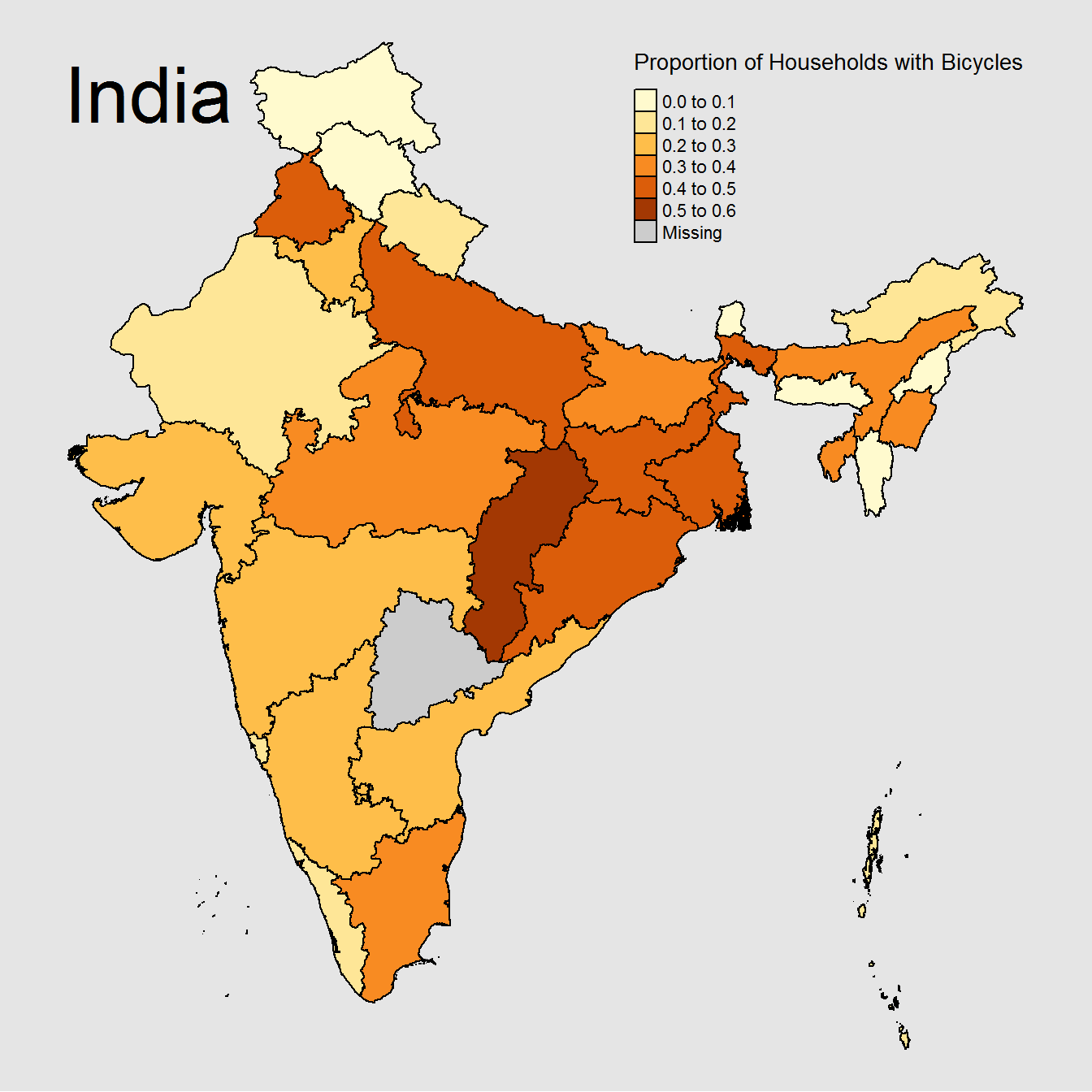
Conclusion
We will leave it to the reader to come up with there own conclusions about some of our graphs above. Still, we clearly have quite a few interesting bits of data from just the few variables we have chosen to graph. For example, biking seems very popular across the country especially in Chhattisgarh. The literacy rate goes down to as low as 50% in some regions, and having internet in a household does not appear to be common. Of course this data is from 2011. So things have likely changed significantly since then. With a new census coming in 2021, there will be opportunities for those interested to look at how this data changes over time (whenever that data becomes available).
In addition to the value of the data itself, we now have more insight into how this data can be utilized for making better machine learning models. For example we might consider treating States and Union Territories differently.
From a data analysis perspective it might also be interesting to find similar data from other countries and make comparisons. For example, could we find similar data from India’s Neighbor Pakistan? What about the United States?