The focus for this topic is to illustrate the usefulness of PCA (Principal Component Analysis) when applied to real world data. As with previous posts in this series we continue to use the 2011 India Census data from Kaggle at https://www.kaggle.com/danofer/india-census. Our goal this time is to classify districts in India by their State.name. We will fit a multinomial logistic regression model and compare predictive accuracy based on a varying number of principal components used to fit the model.
Below we show a list of the packages used.
# packages used
library(here)
library(dplyr)
library(nnet)  # for multinomial functionality
library(reshape2)
library(ggplot2)
We load up our census data as usual.
india_census_data <- here("csv", "kaggle_2020_dec_project",
                          "india-districts-census-2011.csv") %>%
    read.csv()
We now convert the State.name column of our dataframe into a factor and print the levels. We will use this variable as the response variable for our model. The levels correspond to states and territories of India. We have 35 unique states and territories.
india_census_data$State.name <- as.factor(india_census_data$State.name)
print(levels(india_census_data$State.name))
## [1] "ANDAMAN AND NICOBAR ISLANDS" "ANDHRA PRADESH"
## [3] "ARUNACHAL PRADESH" "ASSAM"
## [5] "BIHAR" "CHANDIGARH"
## [7] "CHHATTISGARH" "DADRA AND NAGAR HAVELI"
## [9] "DAMAN AND DIU" "GOA"
## [11] "GUJARAT" "HARYANA"
## [13] "HIMACHAL PRADESH" "JAMMU AND KASHMIR"
## [15] "JHARKHAND" "KARNATAKA"
## [17] "KERALA" "LAKSHADWEEP"
## [19] "MADHYA PRADESH" "MAHARASHTRA"
## [21] "MANIPUR" "MEGHALAYA"
## [23] "MIZORAM" "NAGALAND"
## [25] "NCT OF DELHI" "ORISSA"
## [27] "PONDICHERRY" "PUNJAB"
## [29] "RAJASTHAN" "SIKKIM"
## [31] "TAMIL NADU" "TRIPURA"
## [33] "UTTAR PRADESH" "UTTARAKHAND"
## [35] "WEST BENGAL"Our goal is to predict the State.name, that is the state or territory, in our data. To do this we will split the data into training and testing sets. Since we have many categories for State.name we need to ensure that our training set contains observations with at least 1 instance of each category. To accomplish this we group our data by State.name before taking 60% of the data for our training set for each group. This will ensure our model is trained on each category. Unfortunately, we cannot ensure our model will be tested on each category due to scarcity of some response variables. This is due to the fact that observations are based on district names and sometimes a State.name only corresponds to a single district.
The next few blocks of code are utilized to split our data into training and testing sets. We further divide the data between our response variable and covariates with y referring to our response and X referring to our covariates.
set.seed(123)
training_set <- india_census_data %>%
    dplyr::group_by(State.name) %>%
    dplyr::sample_frac(size=0.6)
training_index <- training_set$District.code
testing_set <- india_census_data[-training_index, ]
# remove District.code and District.name columns
training_set <- subset(training_set, select=-c(1,3))
testing_set <- subset(testing_set, select=-c(1,3))y_train <- training_set["State.name"]
X_train <- subset(training_set, select=-1) # remove State.name
y_test <- testing_set["State.name"]
X_test <- subset(testing_set, select=-1) # remove State.nameNow that are data is split into training and testing sets we would like to apply a multinomial logistic regression model to our data. Doing this on the raw data is problematic due to the high number of covariates and multicolinearity. For example, we start with 115 covariates and have highly correlated variables such as the Population, Male (population of males), and Female (population of females). This is where PCA becomes useful.
Using pca_function from our previous post we can quickly apply PCA to our training set. We we fit our model using 2 to 20 principal components based on our training set and compare the results. The following code shows our process of training and then testing our models. We are using the multinom function from the nnet package to fit the multinomial logistic regression models. Once we have fitted our models, we use the corresponding projection matrix from PCA to transform the original covariates of our testing set to instead be in terms of our principal components. Using this data we predict our response variables and then compare our estimated response variables to the actual testing set values.
# find k-dimensional PC representation of X_train for k=1, 10
# then fit neural network multinomial model with 100 iterations

k <- 20
prediction_accuracy <- rep(0, k)
information_kept <- rep(0, k)
model_aic <- rep(0, k)
for (i in 2:k){
    output <- pca_function(X_train, i, model="fixed", full=TRUE)
    projection_matrix <- output[[1]]
    pca_representation <- scale(X_train) %*% projection_matrix
    pca_training_set <- data.frame(y_train, pca_representation)

    pca_model <- nnet::multinom(State.name ~., data=pca_training_set)
    model_aic[i] <- pca_model$AIC

    pca_testing_set <- data.frame(scale(X_test) %*% projection_matrix)
    pca_predict <- predict(pca_model, newdata=pca_testing_set)

    prediction_accuracy[i] <- mean(pca_predict == y_test$State.name)
    information_kept[i] <- output[[3]]
}
In the above block we kept track of our predictive accuracy, how much information due to variance we kept after applying our PCA model, and the AIC (Akaike information criterion) for each model. We first graph our AIC results.
aic_df <- data.frame(AIC=model_aic[2:20], index=2:20)

ggplot(aic_df, aes(x=index, y=AIC)) +
    geom_point() +
    ggtitle("AIC based on Principal Components Used") +
    xlab("Number of Principal Components")
We can see from these results that our AIC is lowest when we fit our model with 9 principal components. If this were all the information we had to work with, then we would likely choose to use the model with 9 principal components for future predictions. However, since we split our data into training and testing sets we can also judge our models’ performance by considering how the number of principal components used to train our models affect predictive accuracy on our testing set. We have a graph illustrating this below.
plot_df <- data.frame(Accuracy=prediction_accuracy[2:20],
                      Information=information_kept[2:20],
                      index=2:20)
melt_plot_df <- melt(plot_df, id.vars="index")

# plot(plot_df)
ggplot(melt_plot_df, aes(x=index, y=value)) +
    geom_point(aes(shape=variable, color=variable)) +
    ggtitle("Predictive Accuracy and Information kept per PCA Variable") +
    xlab("Number of Principal Components") + ylab("Proportion") +
    labs(color="New Legend Title", shape="New Legend Title") +
    geom_label(
        label=sprintf("(%s, 11)", round(max(prediction_accuracy), 3)),
        x=11+1.8,
        y=max(prediction_accuracy)+.03,
        fill="grey"
        )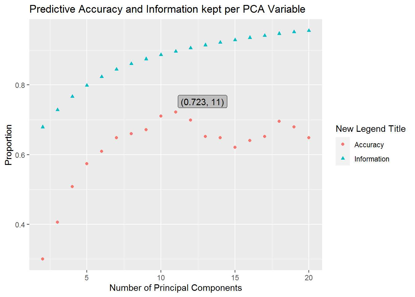
As we can see our predictive accuracy for the number of principal components we keep reaches a maximum at 11 principal components. This shows us that we have a predictive accuracy of 0.7226562 when we keep 11 principal components. Notice that another spike occurs when our model uses 18 principal components, however, it corresponds to lower predictive accuracy and our model works harder to get an estimate due to an increase in variables to consider. Additionally, this second spike is far from our AIC minimum and should likely be avoided.
Overall we can see that PCA keeps most of the important information from a model, removes multicolinearity, and allows for quicker computations. We were able to do all of this while accomplishing the goal of increased predictive accuracy.
Further improvements in our process could be utilized which could both increase predictive accuracy and help ensure predictive accuracy is more consistent for deviations in our training set. To increase predictive accuracy we could try to fully utilize the parameters in the nnet function. To ensure we are really working with a situation where 11 principal components kept is the best choice, we could check alternative training and testing sets or try to implement some form of cross-validation. We note that due to scarcity of some response variables and our limited sample size, certain techniques would be difficult to implement.