Word Cloud - The Republic

For this post we do will create a word cloud of Plato’s The Republic in R using the wordcloud and wordcloud2 packages. The English translation for this work is done by Benjamin Jowett and the data is hosted by MIT at link.

To create the word cloud we first download the text file. Once we have the file, we perform basic data cleaning steps as outlined in the article at link. We then create a data frame with the frequency of words in The Republic and display a table with the 20 most frequent words and follow this up with word clouds. One word cloud for each package. We follow the guide at link. Note that we include the full translation of the Republic including the introduction which was not written by Plato.

We now load the data and create a corpus.

# load raw data and create corpus
raw_data <- readLines(here::here("csv", "republic.mb.txt"))
corpus_data <- Corpus(VectorSource(raw_data))

In this chunk we do the bulk of our data cleaning to remove extremely common words like “a” or “the” as well as remove symbols and other things which are not words.

# clean the data

# convert text to lowercase
corpus_data <- tm_map(corpus_data, content_transformer(tolower))

# remove symbols
corpus_data<-tm_map(corpus_data, content_transformer(gsub),
                    pattern="\\W",replace=" ")

# remove URLs
removeURL <- function(x) gsub("http[^[:space:]]*", "", x)
corpus_data <- tm_map(corpus_data,
                      content_transformer(removeURL))

# remove everything besides English letters or a space
removeNumPunct <- function(x){
    gsub("[^[:alpha:][:space:]]*", "", x)
}
corpus_data <- tm_map(corpus_data,
                      content_transformer(removeNumPunct))

# remove stop words (basic words like "a" and "the")
corpus_data <- tm_map(corpus_data, removeWords,
                      stopwords("english"))

# Code for custom stop words 
# stopwords <- c(setdiff(stopwords('english'),
#                c("r", "k")), "zoo")
# corpus_data <- tm_map(corpus_data, removeWords, stopwords)


# remove extra white space
corpus_data <- tm_map(corpus_data, stripWhitespace)

# remove numbers
corpus_data <- tm_map(corpus_data, removeNumbers)

# remove punctuation
corpus_data <- tm_map(corpus_data, removePunctuation)

In this chunk we use the SnowballC package to perform stemming. This combines similar words to a root form. This may appear a bit unusual with words like “nature” becoming “natur”.

# combines words with multiple spelling types
corpus_data <- tm_map(corpus_data, stemDocument)

We now take our corpus and create a data frame with the words and their frequency.

terms_matrix <- as.matrix(TermDocumentMatrix(corpus_data))
freq_matrix <- data.frame(word=rownames(terms_matrix),
                          freq=rowSums(terms_matrix),
                          row.names=NULL)

From this data frame we list our 20 most common words.

knitr::kable(arrange(freq_matrix, desc(freq))
             %>% head(20))

word	freq
will	1155
said	1047
one	608
true	489
say	489
state	459
good	452
yes	448
may	420
man	374
like	362
natur	310
must	298
can	285
certain	280
now	272
repli	267
thing	266
just	247
also	242

We now create our first word cloud with the wordcloud package.

set.seed(123)
wordcloud(words=freq_matrix$word, freq=freq_matrix$freq,
          min.freq=1, max.words=200, random.order=FALSE,
          rot.per=0, colors=brewer.pal(8, "Dark2"))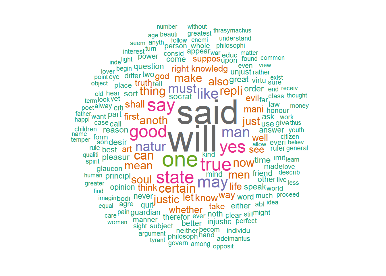

We now conclude our post with a triangular shaped word cloud using the wordcloud2 package.

wordcloud2(freq_matrix, shape = "triangle")