Introduction
For this project we will look at a subsection of data from the weather data available from Kaggle at https://www.kaggle.com/selfishgene/historical-hourly-weather-data. The data includes hourly data from October 2012 to November 2017. We will focus exclusively on the temperature data given in Kelvin (K) for Saint Louis.
We have two objectives for this project. Firstly, we will aggregate the data by day in order to do a two year forecast based on our best model. Secondly, we will aggregate our data by hour and perform a one week forecast based on our best model.
For model selection we will primarily focus on dynamic harmonic regression. For choosing the best model we will split the data into testing and training sets and choose the model with the lowest error.
Section 1
In this first section we are focused on forecasting the daily temperature. We start with data cleaning and then visualize the data. Next we split the data into training and testing sets. We then compare various models against each other. Finally we choose the best model to forecast two years into the future beyond the dataset that we have.
We now load our dataset into R and create an xts object.
# full temperature dataset
temperature <- read.csv(here::here("csv", "kaggle_temperature.csv"), as.is = TRUE)
# saint louis temperature dataset truncated to ignore hours
saint_louis <- xts(x=temperature$Saint.Louis, order.by = as.Date(temperature$datetime))
We next aggregate our data using the mean function for each day.
# deteremines daily mean temperature for saint_louis
# uses split-lapply-as.xts framework
daily_split <- split(saint_louis, f = "days")
means_of_split <- unlist(lapply(daily_split, FUN = mean, na.rm = TRUE))

# create xts and ts
saint_louis_daily_xts <- xts(x = means_of_split, order.by = unique(index(saint_louis)))
saint_louis_daily_ts <- ts(data = means_of_split, start = decimal_date(start(saint_louis_daily_xts)), frequency = 365)
We now include a plot of our daily data.
# displays daily temperature averages for saint_louis
plot.xts(saint_louis_daily_xts,
         main = "Saint Louis average temperature in Kelvin")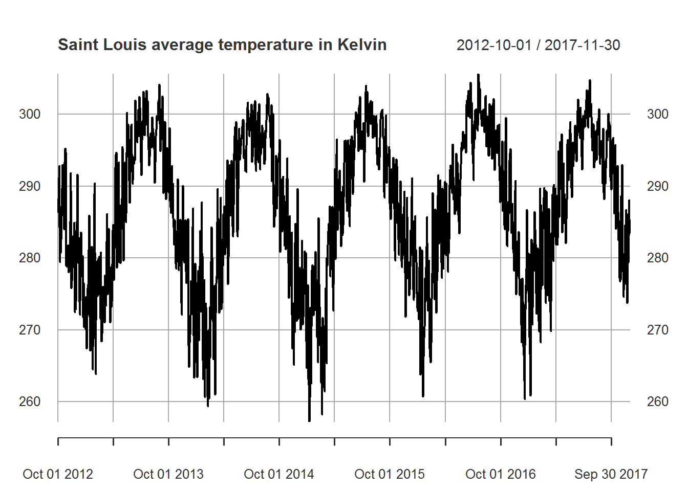
As we can see out data is clearly seasonal. Since we want to forecast a year ahead with daily observations we cannot rely on regular methods of seasonality. In this case we will consider dynamic harmonic regression using \(K=1\) to \(K=10\) Fourier sine and cosine pairs.
Our next chunk of code splits our data into training and testing sets. Using these we use auto.arima to fit our dynamic harmonic regression models to the training sets. Finally we create a matrix of error terms based on comparing our forecasted values to the actual values in our testing sets. We consider Mean Absolute Error (MAE), Root Mean Squared Error (RMSE), and Mean Absolute Percentage Error (MAPE).
# splits data into training and testing sets using dates
train_xts <- saint_louis_daily_xts["2012-10-01/2016-11-30"]
test_xts <- saint_louis_daily_xts["2016-12-01/2017-11-30"]
# uses split xts data to create split ts data for forecasting
train_ts <- ts(data = train_xts, start = decimal_date(start(train_xts)), frequency = 365)
test_ts <- ts(data = test_xts, start = decimal_date(start(test_xts)), frequency = 365)


# loops over harmonic models k=1 to k=10 to find best fit
# uses auto.arima
n=10
error_matrix <- matrix(0L, nrow = n, ncol = 3)
for (k in 1:n) {
  test_harmonics <- fourier(train_ts, K = k)
  fit <- auto.arima(train_ts, xreg = test_harmonics, seasonal = FALSE)
  new_harmonics <- fourier(train_ts, K = k, h = length(test_ts))
  fc <- forecast(fit, xreg = new_harmonics)

  error_matrix[k, 1] <- mean(abs(c(test_ts[,1]) - fc$mean)) # MAE
  error_matrix[k, 2] <- sqrt(mean((c(test_ts) - fc$mean)^2)) # RMSE
  error_matrix[k, 3] <- mean(abs(c(test_ts) - fc$mean) / c(test_ts)) #MAPE
}

# column and row names for error matrix
colnames(error_matrix) <- c("MAE", "RMSE", "MAPE")
rownames(error_matrix) <- c("k=1", "k=2", "k=3", "k=4", "k=5",
                            "k=6", "k=7", "k=8", "k=9", "k=10")
We now examine the results of our models based on the error estimates.
# print error matrix for comparison
error_matrix
## MAE RMSE MAPE
## k=1 4.093070 5.052790 0.01436256
## k=2 4.142757 5.133273 0.01455198
## k=3 4.214339 5.240658 0.01480552
## k=4 4.224612 5.274641 0.01485116
## k=5 4.240699 5.286614 0.01489898
## k=6 4.249974 5.289258 0.01493076
## k=7 4.288388 5.335606 0.01506442
## k=8 4.251684 5.348711 0.01493882
## k=9 4.264996 5.366880 0.01498828
## k=10 4.267089 5.369682 0.01499795Based on these results the dynamic harmonic regression model with \(K=1\) has the lowest error estimates. So we use this model in the chunk below to forecast two years into the future. Our code for this is below.
# uses best prediction model based on error matrix
# forecast unobserved observations
test_harmonics <- fourier(saint_louis_daily_ts, K = 1)
fit <- auto.arima(saint_louis_daily_ts, xreg = test_harmonics, seasonal = FALSE)
new_harmonics <- fourier(saint_louis_daily_ts, K = 1, h = 365*2)
fc <- forecast(fit, xreg = new_harmonics)
We check our residuals for this model below.
# check residiuals
checkresiduals(fit)
##
##  Ljung-Box test
##
## data:  Residuals from Regression with ARIMA(0,1,4) errors
## Q* = 403.24, df = 371, p-value = 0.1199
##
## Model df: 6.   Total lags used: 377
Based on these results we can argue that our residuals are white noise as desired. Finally, we plot our forecast from this model with 80 and 95 percent prediction intervals.
# plot forecast
autoplot(fc) +
  xlab("Date") +
  ylab("Temperature in Kelvin")
Section 2
In this section our goal is to forecast a week ahead using hourly data. We will restrict our study to the temperatures in November 2017 due to the large amount of data present. As with the daily data we split our data into training and testing sets. We choose the best model based on the model with the lowest error terms when measuring our forecasts against the actual values. We then use the best model to forecast one week ahead beyond our given data.
We begin by extracting the data for November and plotting the result.
# create datetime index which includes hourly data
temperature$datetime <- as.POSIXct(strptime(temperature$datetime, "%Y-%m-%d %H:%M:%S"))
temperature_sl <- temperature[, c("Saint.Louis", "datetime")]
# remove times (removes ambiguous times which became NA due to dls?)
temperature_sl <- na.omit(temperature_sl)

# create xts with remaining observations
temperature_sl_xts <- xts(x=temperature_sl$Saint.Louis, order.by = temperature_sl$datetime)
# extract the month of november for forecasting (numbers worked, but check again for dls)
temp_nov_hourly <- temperature_sl_xts["2017-11"]
# plot data
plot.xts(temp_nov_hourly,
         main = "Saint Louis hourly temperature in Kelvin")
While the data above seems almost random, it is clear that the temperature tends to stay relatively close to the previous value. Additionally, we see many deliberate upward and downward trends likely related to the day and night cycle.
We now move on to splitting the data into training and testing sets. We try 12 dynamic harmonic regression models as well as a regular seasonal model. Each model is determined by the auto.arima function. Below we have the code to create our training and testing sets as well as to determine the error between actual and forecasted results for the 12 dynamic regression models.
# split data into test and train
temp_nov_train <- temp_nov_hourly[1:(length(temp_nov_hourly)-24*7), ]
temp_nov_test <- temp_nov_hourly[(length(temp_nov_hourly)-24*7+1):length(temp_nov_hourly), ]

# create ts with appropriate hourly frequency
temp_nov_train_ts <- ts(data=temp_nov_train, frequency=24)
temp_nov_test_ts <- ts(data=temp_nov_test, start = c(23, 2), frequency=24)

# test all possible k values for best harmonic model
n=12
error_matrix <- matrix(0L, nrow=n, ncol=3)
for (k in 1:n) {
  test_harmonics <- fourier(temp_nov_train_ts, K=k)
  fit <- auto.arima(temp_nov_train_ts, xreg=test_harmonics, seasonal=FALSE)
  new_harmonics <- fourier(temp_nov_train_ts, K=k,h =length(temp_nov_test_ts))
  fc <- forecast(fit, xreg=new_harmonics)

  error_matrix[k, 1] <- mean(abs(c(temp_nov_test_ts[,1]) - fc$mean)) # MAE
  error_matrix[k, 2] <- sqrt(mean((c(temp_nov_test_ts) - fc$mean)^2)) # RMSE
  error_matrix[k, 3] <- mean(abs(c(temp_nov_test_ts) - fc$mean) / c(temp_nov_test_ts)) #MAPE
}
colnames(error_matrix) <- c("MAE", "RMSE", "MAPE")
rownames(error_matrix) <- c("k=1", "k=2", "k=3", "k=4", "k=5",
                            "k=6", "k=7", "k=8", "k=9", "k=10",
                            "k=11", "k=12")
Here we print out the error matrix with consideration for MAE, RMSE, and MAPE.
error_matrix## MAE RMSE MAPE
## k=1 12.60621 13.73730 0.04418098
## k=2 12.07566 13.20359 0.04231449
## k=3 11.88865 13.03194 0.04165278
## k=4 11.78077 12.93248 0.04127117
## k=5 11.53285 12.69893 0.04039517
## k=6 11.53641 12.70215 0.04040778
## k=7 11.39093 12.57012 0.03989292
## k=8 11.36152 12.54335 0.03978887
## k=9 11.31491 12.50105 0.03962392
## k=10 11.24324 12.43578 0.03937038
## k=11 11.22534 12.41947 0.03930704
## k=12 11.13907 12.34032 0.03900194In this case we can see that the dynamic harmonic regression model with K=12 has the lowest errors. Before we select this as our model, however, we also consider a seasonal model. We use auto.arima again and allow for seasonality. We print out the resulting errors below:
# also consider seasonal model
fit <- auto.arima(temp_nov_train_ts, seasonal = TRUE)
fc <- forecast(fit, h = 7*24)

seas_error <- matrix(0L, nrow=1, ncol=3)
seas_error[1] <- mean(abs(c(temp_nov_test_ts[,1]) - fc$mean)) # MAE
seas_error[2] <- sqrt(mean((c(temp_nov_test_ts) - fc$mean)^2)) # RMSE
seas_error[3] <- mean(abs(c(temp_nov_test_ts) - fc$mean) / c(temp_nov_test_ts)) #MAPE

colnames(seas_error) <- c("MAE", "RMSE", "MAPE")
rownames(seas_error) <- c("Seasonal")
seas_error
## MAE RMSE MAPE
## Seasonal 15.13771 16.62568 0.05300823This seasonal model clearly has worse error estimates. Before we move on we take a closer look at the residuals for this seasonal model as well as plot the forecast against the actual values.
checkresiduals(fit)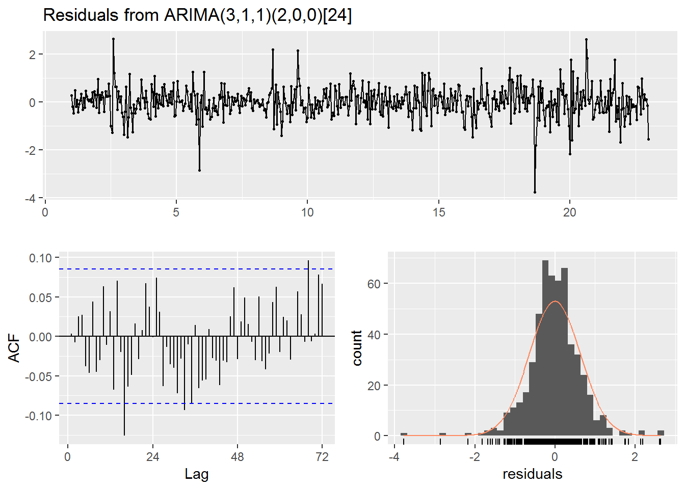
##
##  Ljung-Box test
##
## data:  Residuals from ARIMA(3,1,1)(2,0,0)[24]
## Q* = 63.424, df = 42, p-value = 0.01795
##
## Model df: 6.   Total lags used: 48
autoplot(fc) +
autolayer(temp_nov_test_ts, series = "Data") +
autolayer(fc$mean, series = "Forecast") +
guides(colour=guide_legend(title="Data series")) +
xlab("Day beginning November 1, 2017") +
ylab("Temperature in Kelvin")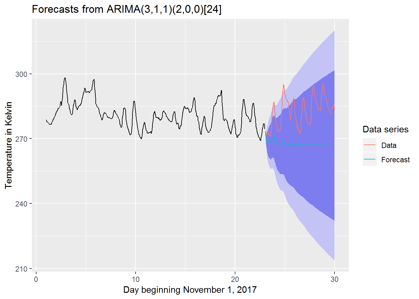
Focusing on the plot we can see that the model is doing a very poor job predicting the actual data. Indeed, while the model does have have a period of 24 it does not seem to utilize that in the predictions which quickly flatten out over time.
We now consider the residuals and forecast for the model with K=12.
# best model
test_harmonics <- fourier(temp_nov_train_ts, K = 12)
fit <- auto.arima(temp_nov_train_ts, xreg = test_harmonics, seasonal = FALSE)
new_harmonics <- fourier(temp_nov_train_ts, K = 12, h = 7*24)
fc <- forecast(fit, xreg = new_harmonics)

checkresiduals(fit)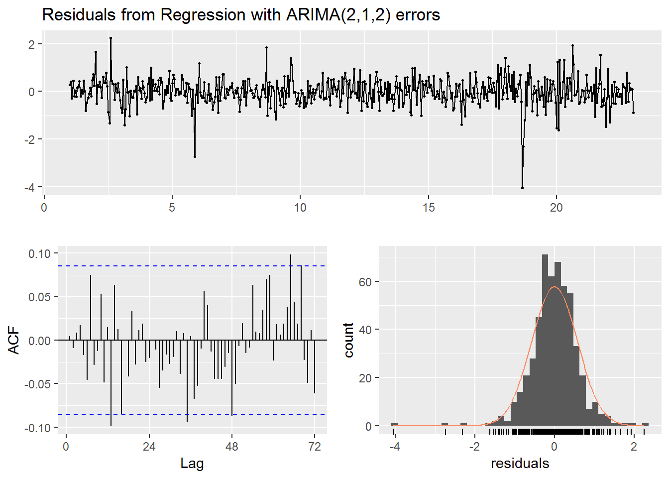
##
##  Ljung-Box test
##
## data:  Residuals from Regression with ARIMA(2,1,2) errors
## Q* = 47.36, df = 21, p-value = 0.0008397
##
## Model df: 27.   Total lags used: 48
autoplot(fc) +
autolayer(temp_nov_test_ts, series = "Data") +
autolayer(fc$mean, series = "Forecast") +
guides(colour=guide_legend(title="Data series")) +
xlab("Day beginning November 1, 2017") +
ylab("Temperature in Kelvin")
Based on the low p-value from the Ljung-Box test we should be wary of our predictions. On the other hand if we consider the graphs of our residuals it does seem that the results are mostly uncorrelated and follow a roughly normal distribution. Slightly more concerning is the fact that while the forecast does a decent job of predicting the up and down motion of the day it does not seem take into account the larger spikes from the older data and that is likely why it fails to adequately pick up the large spikes in the actual data. Still, unlike with the previous seasonal model the data does stay within the 95% prediction interval.
We now move to forecasting one week into the future using out best hourly forecasting model.
# hourly forecast into the unknown
temp_nov_hourly <- ts(data=temp_nov_hourly, frequency=24)

test_harmonics <- fourier(temp_nov_hourly, K = 12)
fit <- auto.arima(temp_nov_hourly, xreg = test_harmonics, seasonal = FALSE)
new_harmonics <- fourier(temp_nov_hourly, K = 12, h = 7*24)
fc <- forecast(fit, xreg = new_harmonics)

checkresiduals(fc)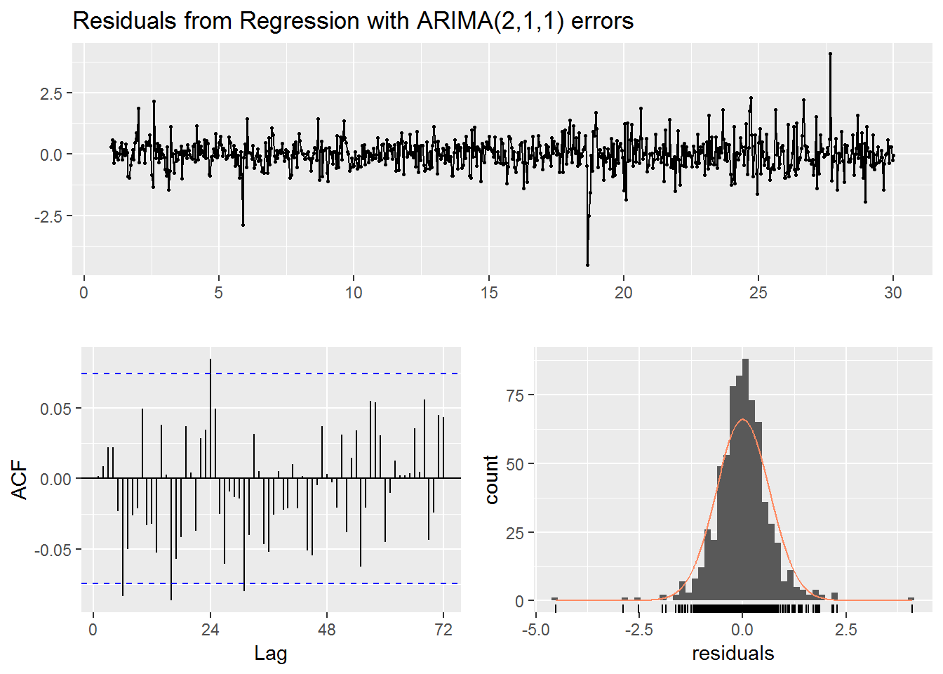
##
##  Ljung-Box test
##
## data:  Residuals from Regression with ARIMA(2,1,1) errors
## Q* = 54.546, df = 22, p-value = 0.0001378
##
## Model df: 26.   Total lags used: 48
autoplot(fc) +
xlab("Day beginning November 1, 2017") +
ylab("Temperature in Kelvin")
As with the previous instance the Ljung-Box test has a small p-value, but graphically the residuals appear uncorrelated and normally distributed. The forecast itself seems to have smaller daily ups and downs compared to the rest of the data. So there could be improvement for the forecast, but ultimately we do not know the true values. Technically we could look up the true values now. Still, as with the previous situation we can be fairly confident in our 80% and 95% prediction intervals which did contain the actual observations when we were able to compare to the actual data.
Conclusion
In the case of our one year daily forecast our model, while technically simple, seems to be about as reasonable as possible given what we know. Indeed, the model was able to pick up the general seasonal trend that occurs throughout the year, but none of the finer details. This seems to be about the best we can expect, however, we could also try to determine without seasonality if the temperature is rising or falling year over year.
In the case of our hourly forecast it appears that our model does a decent job predicting the daily up and down cycle, however, from visual comparison of the forecast with the actual data it may be possible to do a little better. Perhaps we could look beyond simply applying auto.arima and find an appropriate transformation of the data to ensure model variation is more consistent.