In this post we will be examining data from the Zillow Home Value Index (ZHVI) for Missouri available at https://www.zillow.com/mo/home-values/. Unlike some value indexes this data can be interpreted as the median dollar value of the home. We will first look at the values of houses based on the number of rooms and then forecast the value of all houses across the state of Missouri using a dynamic regression model. We will use seasonally adjusted unemployment rates in Missouri for our regression model obtained from the FRED at https://fred.stlouisfed.org/series/MOUR.
Some of the packages used directly in this project include here, readxl, ggplot2, janitor, xts, lubridate, and fpp2. We begin by including code for importing the data from an Excel file and a csv file. We also convert our data into class xts.
# Code for importing data

clean_excel_data <- function(sheet){
  # takes extracted excel path and sheet name and then cleans data
  # according to task specific specification
  suppressMessages(
    cleaning <- read_xlsx(path = here::here("csv",
                          "Zillow_Missouri_Home_Prices.xlsx"),
                          sheet = sheet, skip = 1, col_names = FALSE,
                          col_types = "text")
  )
  cleaning <- t(cleaning)
  cleaning <- cleaning[-c(2,3), ]
  colnames(cleaning) <- cleaning[1, ]
  cleaning <- cleaning[-1, ]
  cleaning <- as.data.frame(cleaning)
  cleaning[] <- lapply(cleaning, as.character)
  cleaning[] <- lapply(cleaning, as.numeric)
  cleaning[, 1] <- excel_numeric_to_date(cleaning[, 1])
  return(xts(x = cleaning[, -1], order.by = cleaning[, 1]))
}

# Imports Zillow Home Value Index data
all_homes_xts <- clean_excel_data(sheet = "All Homes")
one_bed_xts <- clean_excel_data(sheet = "One Bed")
two_bed_xts <- clean_excel_data(sheet = "Two Bed")
three_bed_xts <- clean_excel_data(sheet = "Three Bed")
four_bed_xts <- clean_excel_data(sheet = "Four Bed")
many_bed_xts <- clean_excel_data(sheet = "Many Bed")

# Imports seasonally adjusted Missouri unemployment data from FRED
missouri_unem <- read.csv(here::here("csv", "MOUR.csv"), as.is = TRUE)
missouri_unem_xts <- xts(x = missouri_unem[, 2],
                         order.by = as.Date(missouri_unem[, 1]))
missouri_unem_xts <- window(missouri_unem_xts, start =
                              floor_date(start(all_homes_xts), "month"))
Below we can see that the growth rate of median home values is consistent regardless of the number of rooms. Additionally the median for all homes is close to the median value for homes with 3 bedrooms.
# plot data
zhvi <- cbind(all_homes_xts[, "Missouri"], one_bed_xts[, "Missouri"],
      two_bed_xts[, "Missouri"], three_bed_xts[, "Missouri"],
      four_bed_xts[, "Missouri"],many_bed_xts[, "Missouri"])
colnames(zhvi) <- c("All Homes", "One Bed", "Two Bed", "Three Bed",
                    "Four Bed", "Many Bed")

plot(zhvi, main = "Zillow Home Value Index", legend.loc = "topleft")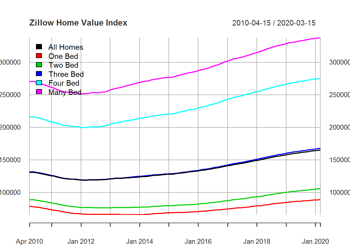
Next we look at the Missouri unemployment rate truncated to the dates we have for our home index values. We have data through April 2020 where we witness a large spike in unemployment.
plot(missouri_unem_xts, main = "Missouri Unemployment Rate")
We now combine the Missouri ZHVI numbers for all homes with the unemployment rate. Additionally, we add data estimates from Zillow for April and May. We use the April rate of 9.7% as an estimate of the May unemployment rate, this is due to a lack of data for Missouri’s unemployment rate in May. We now view our plots with additional data and data estimates below:
zhvi_missouri <- zhvi[,1]
# new data based on visual graph of existing data on Zillow (not exact)
new_data <- xts(x = c(164000,163000),
                order.by = as.Date(c("2020-4-15", "2020-5-15")))
zhvi_missouri <- rbind(zhvi_missouri, new_data)

new_unem <- xts(9.7, order.by = as.Date("2020-5-01")) # guess
# force zhvi dates to beginning of month for consistancy
index(zhvi_missouri) <- floor_date(index(zhvi_missouri), "month")
# merge zhvi and unemployment
full_data <- cbind(zhvi_missouri, rbind(missouri_unem_xts, new_unem))
colnames(full_data) <- c("Value", "Unemployment")

par(mfrow = c(2,1))
plot(full_data[,1], main = "Missouri Zillow Home Value Index")
plot(full_data[,2], main = "Missouri Unemployment Rate", col = "red")
Below we look for the correlation between the unemployment rate and home values.
zhvi_unem_xts <- full_data
zhvi_unem_df <- cbind(Date = index(full_data),
                      as.data.frame(full_data, row.names=FALSE))

ggplot(aes(x = Value, y = Unemployment), data = zhvi_unem_df) +
  geom_point() +
  ggtitle("Visual Check for Correlation")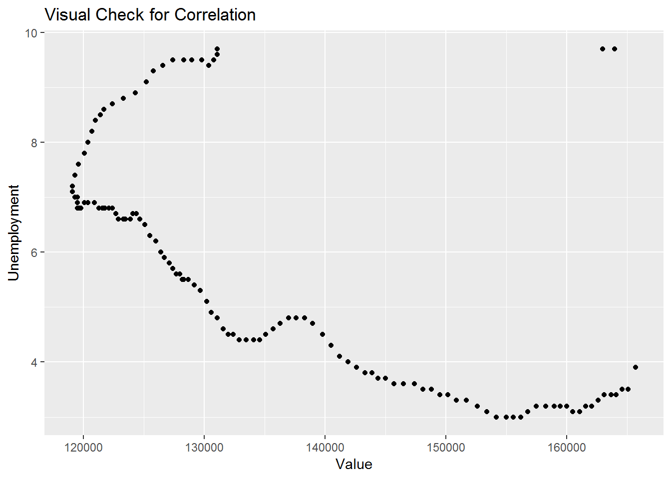
We can see that a relationship does exist and can find the correlation to be -0.6908. We now look into fitting our model. To keep things simple we use auto.arima which automatically determines which type of model to choose.
fit <- auto.arima(zhvi_unem_xts$Value, xreg = zhvi_unem_xts$Unemployment)

checkresiduals(fit)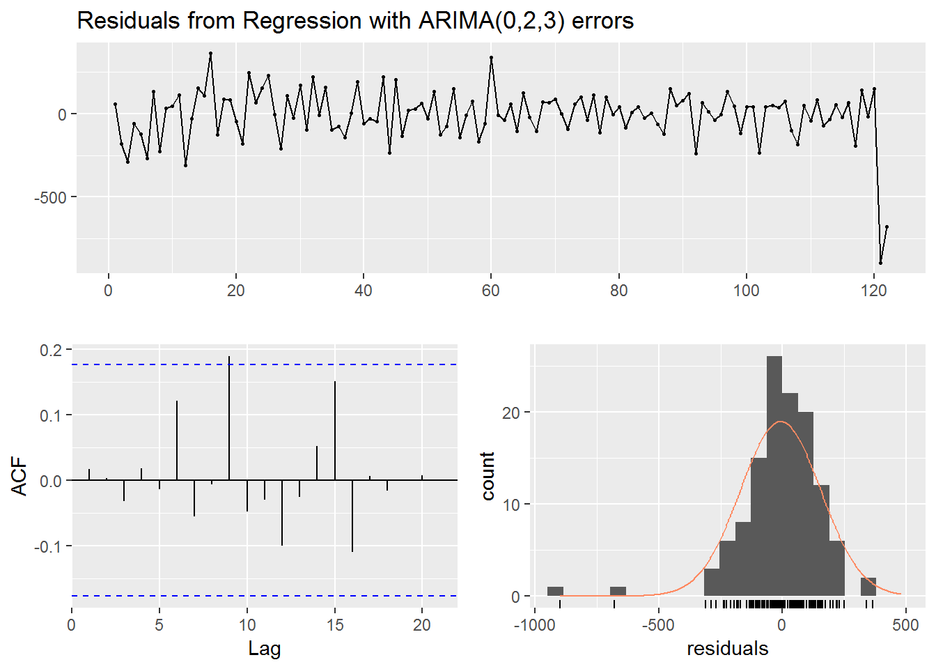
##
##  Ljung-Box test
##
## data:  Residuals from Regression with ARIMA(0,2,3) errors
## Q* = 7.6956, df = 6, p-value = 0.2613
##
## Model df: 4.   Total lags used: 10
As we can see from our check of residuals our data was differenced twice to fit the model. Moreover, we have large negative residual which skew the distribution. Based on the results of the Ljung-Box test we can argue that our model has independently distributed residuals.
We now move into the forecasting stage. We go with a two year forecast. Since we do not know the unemployment rate for that time we simply assume unemployment will stay 9.7% to keep things simple.
xreg_fc <- as.matrix(rep(9.7, 24))
colnames(xreg_fc) <- "Unemployment"

fc <- forecast(fit, xreg = xreg_fc)

autoplot(fc, ylab="ZHVI")
Based on our model our forecast indicates a decrease in home value. Our probability bands do include a small probability that prices will pick back up in the next two years based on the 95% prediction interval. Note that while these predictions seem reasonable there are many factors that have not been taken into full consideration. Unemployment rate for example is highly unpredictable and could easily end up going up or down. Additionally, inflation across the economy could cause prices to increase.