In this post we will do a simple cluster analysis. For our data we will use online sales data which we obtained from the UCI Machine Learning Repository at https://archive.ics.uci.edu/ml/datasets/Online+Retail+II. We will be using the here, readxl, ggplot2 and dplyr packages for this project. In our first chunk we begin by reading our Excel data into R.
# read in the two different Excel sheets
mydata1 <- read_xlsx(path = here::here("csv", "online_retail_II.xlsx"), sheet = 1)
mydata2 <- read_xlsx(path = here::here("csv", "online_retail_II.xlsx"), sheet = 2)

# combines the two datasets
myfulldata <- rbind(mydata1, mydata2) # combines the two data frames
To give our reader some knowledge of our data set we look at the structures of the data:
str(myfulldata)## Classes 'tbl_df', 'tbl' and 'data.frame': 1067371 obs. of 8 variables:
## $ Invoice : chr "489434" "489434" "489434" "489434" ...
## $ StockCode : chr "85048" "79323P" "79323W" "22041" ...
## $ Description: chr "15CM CHRISTMAS GLASS BALL 20 LIGHTS" "PINK CHERRY LIGHTS" "WHITE CHERRY LIGHTS" "RECORD FRAME 7\" SINGLE SIZE" ...
## $ Quantity : num 12 12 12 48 24 24 24 10 12 12 ...
## $ InvoiceDate: POSIXct, format: "2009-12-01 07:45:00" "2009-12-01 07:45:00" ...
## $ Price : num 6.95 6.75 6.75 2.1 1.25 1.65 1.25 5.95 2.55 3.75 ...
## $ Customer ID: num 13085 13085 13085 13085 13085 ...
## $ Country : chr "United Kingdom" "United Kingdom" "United Kingdom" "United Kingdom" ...We can see that we are working with a data frame with 8 variables and over 1 million observations. For our purpose we will focus primarily on the Country, Price and Quantity variables. Note that our earliest order is from 2009-12-01 07:45:00 while our newest order is from 2011-12-09 12:50:00.
We now do some data cleaning. This includes removing rows of data which are exactly identical or involve cancelled orders. We will retain the initial order even if a cancellation was made. This is done for simplicity and due to the fact that newer orders could be cancelled, but not included in our data set.
# data cleaning

duplicates <- which(duplicated(myfulldata)) # determines index of repeated rows
mydata <- myfulldata[-duplicates, ] # full data without duplicates

cancellations <- which(startsWith(mydata$Invoice, "C")) # find cancelled orders
mydata <- mydata[-cancellations, ] # removes order cancellations (retains original order)
Now that we have cleaner data, we aggregate our results by country. This is done by calculating the mean Quantity and Price for each item in a transaction by country. We will also include the total number of item transactions for each country while ignoring the Quantity variable.
countrynames <- unique(mydata$Country) # names of unique countries
n <- length(unique(mydata$Country)) # number of unique countries

# aggregate data by Quantity and Price
agg_sum <- aggregate(mydata[,c(4,6)], by=list(mydata$Country), FUN = mean, na.rm = TRUE)

agg_ct <- mydata%>% group_by(Country) %>% tally() # count of item transactions ignoring Quantity

my_aggregates <- cbind(agg_ct, agg_sum[,2:3]) #combine aggregates
Let’s take a quick look out our aggregate data frame below.
print(my_aggregates)## Country n Quantity Price
## 1 Australia 1792 58.073103 3.586724
## 2 Austria 922 12.557484 4.281681
## 3 Bahrain 124 10.798387 3.479274
## 4 Belgium 3056 11.380236 4.242153
## 5 Bermuda 34 82.294118 2.491176
## 6 Brazil 94 5.797872 2.726702
## 7 Canada 228 16.039474 4.640746
## 8 Channel Islands 1551 13.794971 4.586415
## 9 Cyprus 1136 9.639085 5.124507
## 10 Czech Republic 25 26.840000 3.130800
## 11 Denmark 778 305.232648 2.808483
## 12 EIRE 17159 19.616761 5.459230
## 13 European Community 60 8.316667 4.830000
## 14 Finland 1032 13.929264 4.765698
## 15 France 13640 19.934164 4.272210
## 16 Germany 16440 13.696655 3.590424
## 17 Greece 657 11.756469 3.852024
## 18 Hong Kong 354 19.833333 31.312881
## 19 Iceland 222 13.364865 2.498063
## 20 Israel 366 15.131148 3.578033
## 21 Italy 1442 10.618585 4.782032
## 22 Japan 468 67.613248 2.011154
## 23 Korea 53 13.207547 2.267170
## 24 Lebanon 57 8.035088 5.595439
## 25 Lithuania 154 14.974026 2.564740
## 26 Malta 282 8.932624 13.361773
## 27 Netherlands 5090 75.544008 2.682460
## 28 Nigeria 30 3.433333 3.416000
## 29 Norway 1290 18.312403 15.627814
## 30 Poland 504 11.285714 3.656687
## 31 Portugal 2470 11.222267 5.000623
## 32 RSA 168 11.732143 11.420000
## 33 Saudi Arabia 9 8.888889 2.351111
## 34 Singapore 339 20.631268 39.299410
## 35 Spain 3663 13.736828 4.262738
## 36 Sweden 1336 66.342066 4.911475
## 37 Switzerland 3123 16.894973 3.746929
## 38 Thailand 76 33.578947 2.999605
## 39 United Arab Emirates 467 15.676660 4.298394
## 40 United Kingdom 932030 9.514645 3.819723
## 41 Unspecified 748 8.995989 2.912179
## 42 USA 409 12.870416 3.577237
## 43 West Indies 54 7.314815 2.273519We can see that we are working with 43 difference countries. Notice that some countries have very few transactions (denoted by the n column). We will remove the countries with fewer than 100 item transactions from further analysis.
small_orders <- which(my_aggregates$n < 100)
my_aggregates <- my_aggregates[-small_orders, ] # removes countries with less than 100 orders
We now look at our remaining data in a plot of Quantity and Price.
ggplot(my_aggregates, aes(x = Price, y = Quantity, label = Country)) +
  geom_point() +
  geom_text(aes(label=Country),hjust=0, vjust=0, size = 2) +
  ggtitle("Base Plot")
Now that we know where our data falls in the plot, we need to do a cluster analysis to group the data together. To determine the number of clusters we will look at the within sum of squares and choose the number of centers right before the within sum of squares does not appreciably decline. Below we look at a graph of our within sum of squares:
# run kmeans on data for various numbers of clusters
wss <- (nrow(my_aggregates)-1) * sum(apply(my_aggregates[, c(3,4)], 2, var))
  for ( i in 2:10) wss[i] <- sum(kmeans(my_aggregates[,c(3:4)], centers = i, nstart = 20)$withinss)

plot(1:10, wss, type = "b", xlab = "Number of Clusters", ylab = "Within groups sum of squares")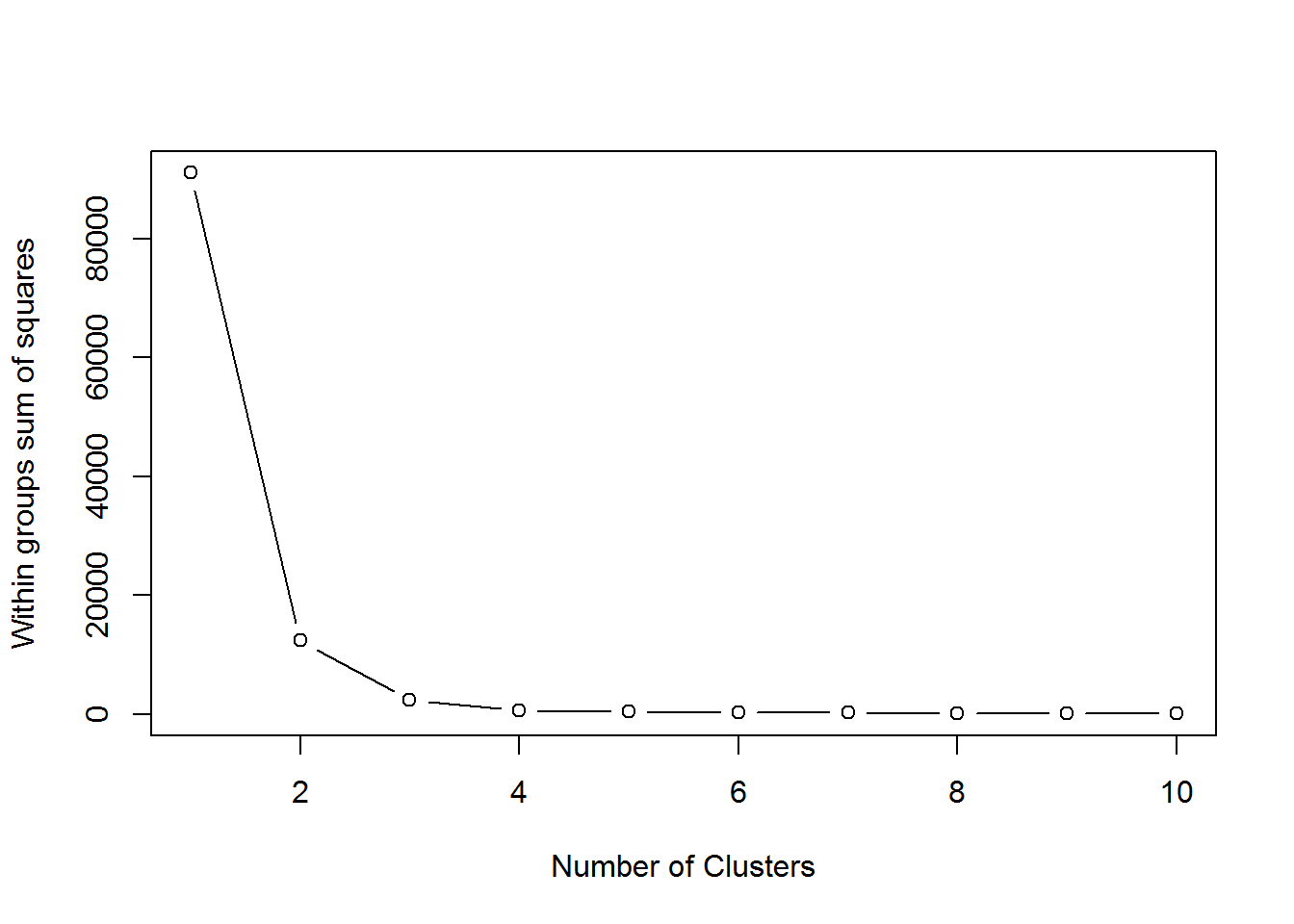
Based on our graph above we may choose either 4 or 5 centers (or clusters). We include results for 4 and 5 clusters below.
set.seed(123)
sc <- kmeans(my_aggregates[,c(3:4)], centers = 4, nstart = 20)
agg_sc <- cbind(my_aggregates, group = sc$cluster)
ggplot(agg_sc, aes(x = Price, y = Quantity, label = Country, col = factor(group))) +
  geom_point()  + theme(legend.position = "none") +
  geom_text(aes(label=Country),hjust=0, vjust=0, size = 3, alpha = 0.8) +
  ggtitle("Plot with 4 Clusters")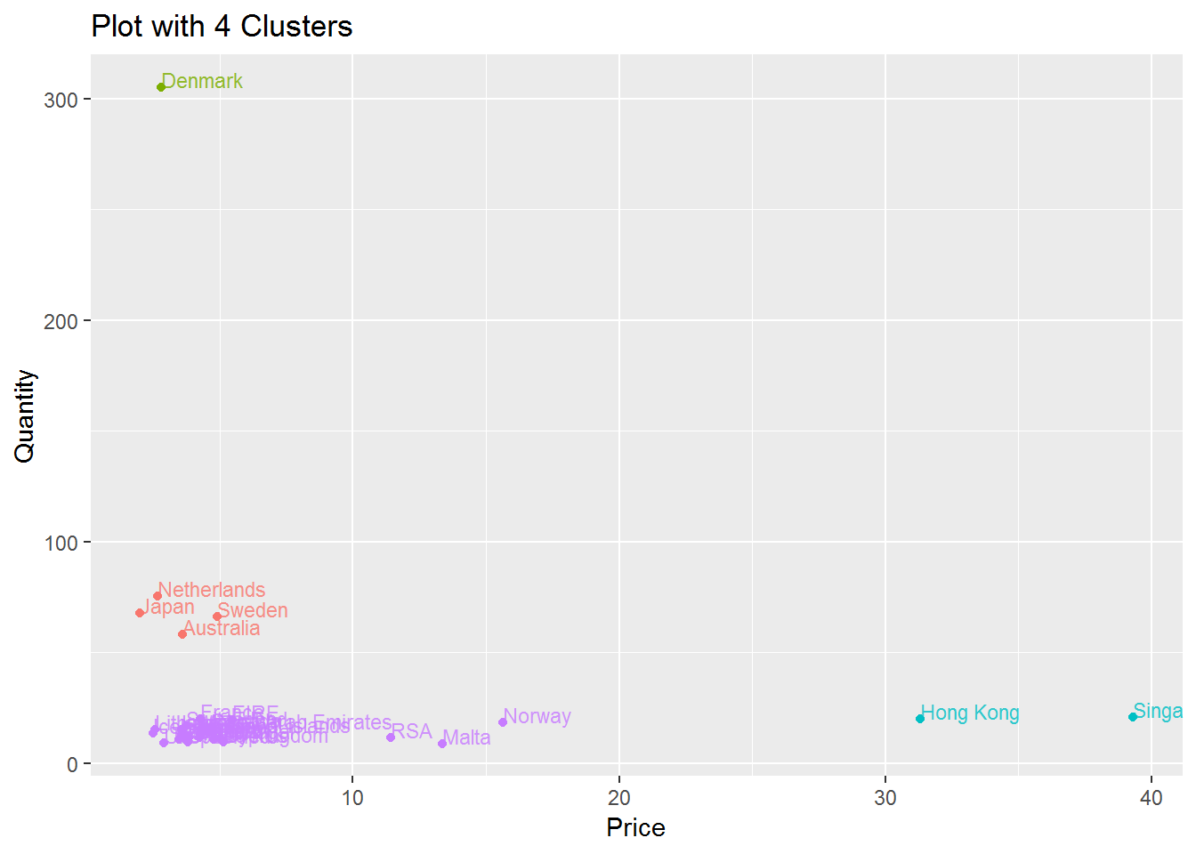
sc <- kmeans(my_aggregates[,c(3:4)], centers = 5, nstart = 20)
agg_sc <- cbind(my_aggregates, group = sc$cluster)
ggplot(agg_sc, aes(x = Price, y = Quantity, label = Country, col = factor(group))) +
  geom_point()  + theme(legend.position = "none") +
  geom_text(aes(label=Country),hjust=0, vjust=0, size = 3, alpha = 0.8) +
  ggtitle("Plot with 5 Clusters")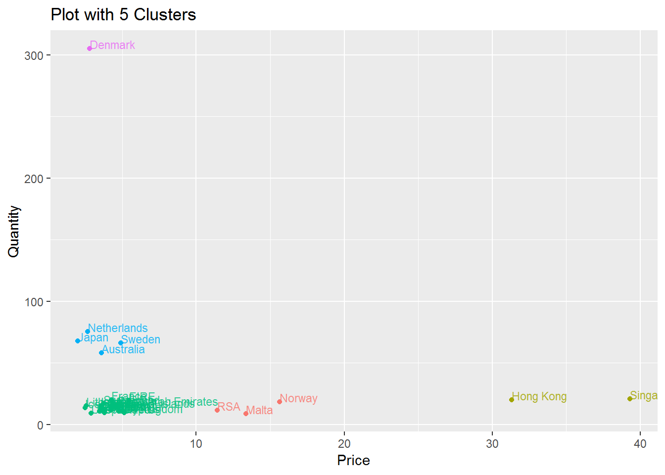
Based on the graphs above, I think having 5 centers is better since it distinguishes RSA, Malta and Norway from the other countries in the bottom left corner.
We conclude with a few results from our graphs. Notably, most countries tend to buy cheap goods in low quantities. Denmark tends to have more goods which are bought in large quantities while Hong Kong and Singapore tend to buy few items that are at a higher price point. To get a better idea why Denmark has such large quantities we can try to search for Quantities that are very high. One order with some very high quantities include Invoice 495194 which we include below:
mydata[mydata$Invoice == "495194",]## # A tibble: 15 x 8
## Invoice StockCode Description Quantity InvoiceDate Price
## <chr> <chr> <chr> <dbl> <dttm> <dbl>
## 1 495194 37410 BLACK AND ~ 6012 2010-01-21 15:11:00 0.1
## 2 495194 16051 TEATIME PE~ 866 2010-01-21 15:11:00 0.06
## 3 495194 16044 POP-ART FL~ 6144 2010-01-21 15:11:00 0.06
## 4 495194 21702 SET 5 MINI~ 2040 2010-01-21 15:11:00 0.3
## 5 495194 17109C FLOWER FAI~ 2520 2010-01-21 15:11:00 0.15
## 6 495194 17109B FLOWER FAI~ 3888 2010-01-21 15:11:00 0.15
## 7 495194 16254 TRANSPAREN~ 864 2010-01-21 15:11:00 0.25
## 8 495194 20889 JARDIN DE ~ 408 2010-01-21 15:11:00 0.3
## 9 495194 20759 CHRYSANTHE~ 5280 2010-01-21 15:11:00 0.1
## 10 495194 20758 ABSTRACT C~ 4800 2010-01-21 15:11:00 0.1
## 11 495194 20757 RED DAISY ~ 4800 2010-01-21 15:11:00 0.1
## 12 495194 20756 GREEN FERN~ 5280 2010-01-21 15:11:00 0.1
## 13 495194 20755 BLUE PAISL~ 4320 2010-01-21 15:11:00 0.1
## 14 495194 20991 JAZZ HEART~ 6768 2010-01-21 15:11:00 0.1
## 15 495194 20993 JAZZ HEART~ 9312 2010-01-21 15:11:00 0.1
## # ... with 2 more variables: `Customer ID` <dbl>, Country <chr>Clearly these values are quite large and are undoubtedly a factor in the large average Quantity for Denmark. From a company perspective it could be beneficial to be aware of some of these bulk buyers. For our own analysis it may be worth double checking our order cancellations to ensure that such a large order is not unfairly biasing our results. In conclusion, we are able to get nice visuals and group countries by Quantity and Price. This is great and we may think that we could just draw circles without the extra statistical analysis, but in general visualization may be very challenging with a higher number of variables and k-means will still work just as well!