Introduction
In this project we will use Dynamic Linear Models (DLMs) to forecast sales figures from five different stores. The dataset we use is a slightly modified version of a dataset derived from Kaggle https://www.kaggle.com/. We explain the exploratory data analysis process in the Project Overview section. We then look at and explain some of the major results. This involves using graphs of the data and our forecasts to try to understand some of the patterns and trends in the data. As part of our results we include a one month forecast with our daily data. Finally, we also include a two year monthly forecast for our data.
Project Overview
The focus for the early part of the project was data cleaning and exploration along with and basic model fitting.
For the data cleaning aspect, we changed the dates from a factor to a POSIXct class. Additionally, we examined certain categorical variables and converted them from integers to factors. We also changed the store data from numbers to factors and labeled the stores A, B, C, D, and E for convenience.
Once initial data cleaning was completed, we took a look at various graphs of the data. Looking at overlapping graphs of the data by store was messy and so we then looked at individual graphs of the data. This indicated that we probably had two types of store. This agrees with the StoreType variable of our data as well. We determine that the two store types correspond to two stores which are always open and three stores which are closed on StateHolidays and on Sunday. As part of our exploration we also look at the sales for each store based on the day of the week.
Model fitting was done using a Dynamic Linear Model (DLM) framework. Various models were considered for different stores and variables. Primarily, a local linear trend model with weekly seasonality was considered with regression on various combinations of variables in order to predict one-step-ahead daily forecasts of sales. We looked at graphs of our predictions against the actual values along with computing error estimates for our forecasts. Note that some values of sales figures and customer counts were not available. The DLM package that we used was able to forecast without concern for the missing data. It simply makes its own prediction for the missing value. For the error estimate, we simply remove NA values from the calculation.
In later portions of our data exploration we look at various factors for each store. We also fit Dynamic Linear Models (DLMs) for the three stores which are closed on Sunday and state holidays. For the factors we analyze the graphs based on characteristics such as Promo, SchoolHoliday and StateHoliday. We also take another look at the stores for each day of the week. Rather than use the days of the week as a factor we simply look at DLMs with weekly seasonality. Finally, we also take a look at error analysis and look at some graphs of the residuals. We do similar data exploration by fitting DLMs to the two stores which are always open.
We next aggregate our data from daily into monthly data. This is done, so that we can make one and two year forecasts focusing on monthly averages for daily sales on days the stores were open. In this case we fit Dynamic Linear Models (DLMs) with local linear trend and monthly seasonality. We look at forecasts for these models and analyze the residuals and error.
We next wanted to figure out the spacing of promotional events and of School Holidays. From our analysis we determined that promotional events are done on the same day for each store while school holidays tend to differ between store.
We next perform one-step-ahead forecasting to predict an entire month of sales values at the daily level. We include covariate data on promotions and whether a store is open to enhance predictions.
Finally, we begin putting everything together and creating nice graphs. Our main results and conclusions will be given in the following sections.
Goals and Dynamic Linear Models
Combining and refining our exploratory results, our goal is to create a convincing argument for actionable business initiatives at both a technical and less technical level. We will be using Dynamic Linear Models (DLMs) for our analysis and forecasting. One major advantage of these models is that they do not require us to worry about transforming our data to make it stationary. Now, the general model of a DLM we will be using is the following: \[y_t = F_t \theta_t + v_t, \ v_t \sim N(0, V_t)\] \[\theta_t = G_t \theta_{t-1} + w_t, \ w_t \sim N(0,W_t)\] \[\theta_0 \sim N(m_0, C_0)\]
The first equation is called the observation equations with \(y_t\) being the observations of the time series. This can be either a scalar or a vector depending on the situation. The second equation is called the state equation where the states are given by \(\theta_t\). Generally, \(\theta_t\) will be a vector, but it can be a scalar for simple models. The state equation is used to keep track of trend, seasonality, and regression values.
Data Exploration
In this section we begin working with the data. We load the data from the source file and then rename variables and change covariate datatypes as needed. Each of our five stores will now be referred to as Store A, Store B, Store C, Store D and Store E. We begin by looking at the raw data for the stores categorized by the day of the week.
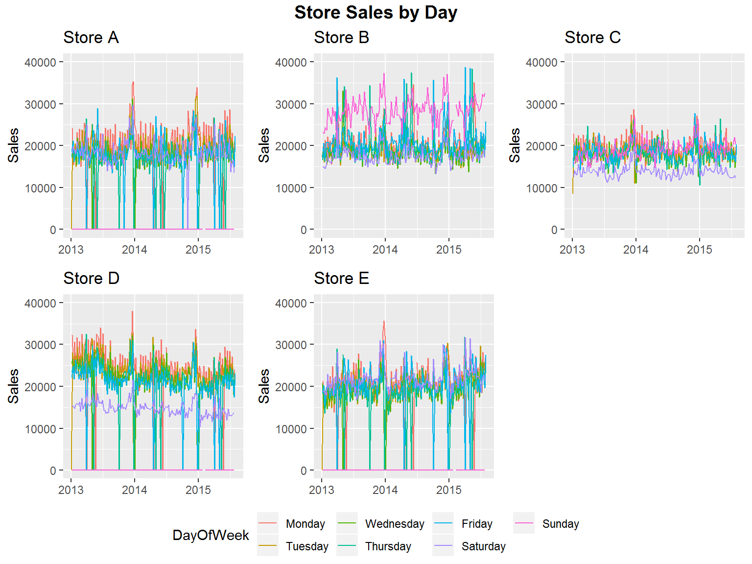
Having looked at the raw data, we see a lot of noise. To fix the issue with the noise we apply the local linear trend DLM to the data based on the day of the week and then smooth our results. We show our results below:

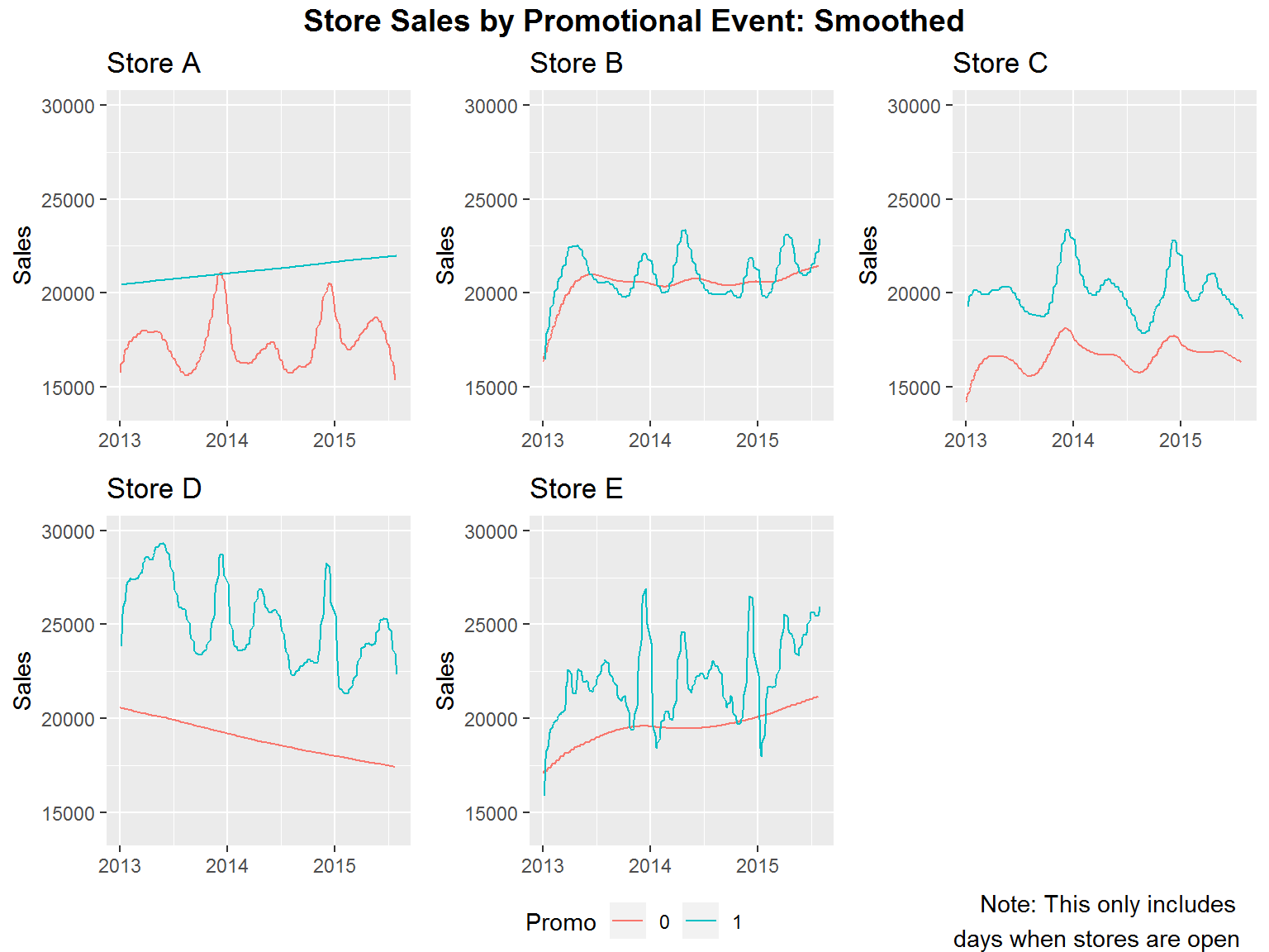
Our next goal is to look at smoothed values for promotional events. We do this first by looking at whether we have a promotional event or not and then smooth the individual time series. We only consider days that the store is open for this result.
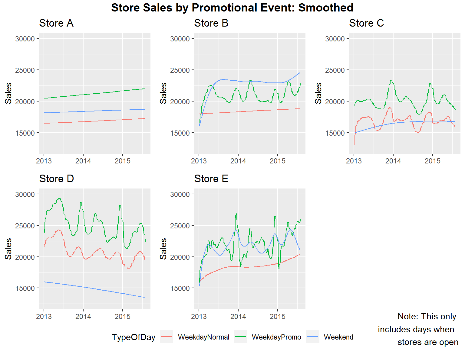
We now look further at promotional events by splitting our data into three categories. From our analysis, we noticed that all stores have promotional events on the exact same days. Additionally, all promotional events are on weekdays Monday through Friday and are consistently every other week. So for days when the stores are open we consider the categories of 1) weekends, 2) weekdays without a promotion going on and 3) weekdays with a promotion going on.
Based on our results for promotions we see some interesting trends. First of all, in four of our five stores we have promotions yielding most or almost most of our highest sales figures. The store which doesn’t fit this very much is store B. This is because store B has really good weekend sales. If we look at our daily sales we can see that specifically, store B has really great Sunday sales figures.
Another bit of data that we were interested in was school holidays. We wanted to see if this had any noticeable affect on sales. Based on the results below it is hard to determine in most cases, however, it does appear that store D has better sales during school holidays than on a regular day. In the other cases it seems mostly inconclusive.

Combining our observations we can say a few things. The day of the week tends to have a reasonable effect on sales. Additionally, promotional events tend to have the highest sales with weekends having the second highest sales and weekdays without promotions having the lowest sales. We also do not see school holidays as a very good predictor since the results tend to be mixed. Finally, there seems to be a general loss in sales over time with store D.
One-Step-Ahead Daily Forecasting
Now that we have finished our initial observations of the data, we try to do forecasting at a daily level. We want to predict one month ahead of our current data in this manner. We use the Dynamic Linear Model (DLM) framework for our model. Our model will have a local linear trend component along with a weekly seasonality component and a regression component. The regression component is based on whether the store is open and whether the store has a promotion.
We do have data on the number of customers at different times, but we do not use regression on that data due to having no idea what those values will be in the future. We could have used a model with NA customer counts for the days we want to predict, but we decided against it. We were able fill in future values of days the stores were open and days the stores have promotions by looking at the historical data and trend.
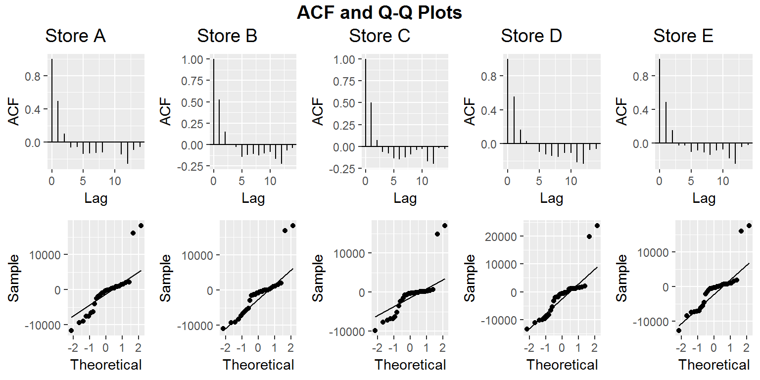
After computing our models we take a look at the Auto Correlation Function (ACF) and Q-Q plots for our residuals. We see this in the figure below.
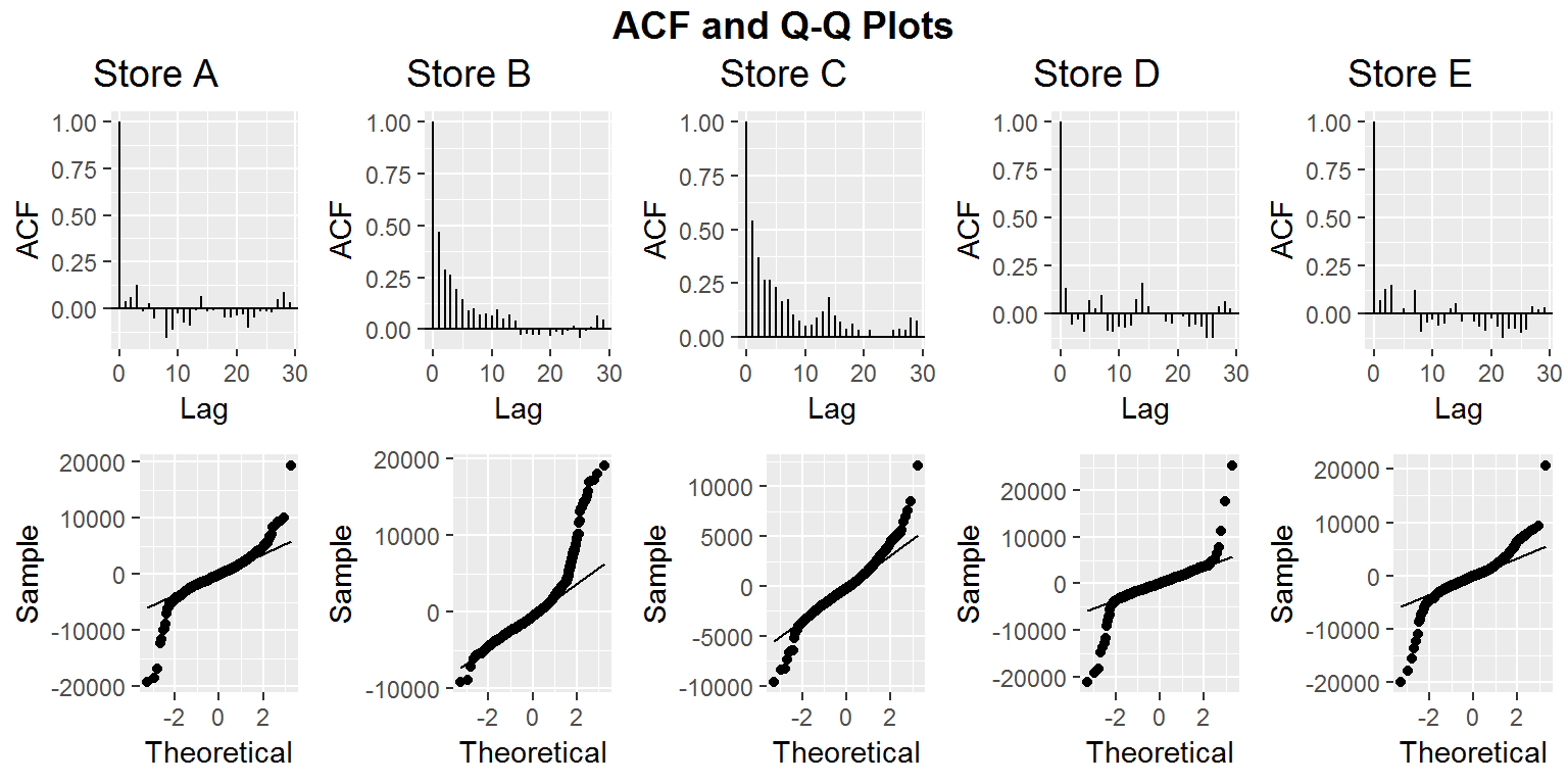
Based on the results for ACF, Store B and Store C residuals may have some correlation that we did not appropriately account for in our model. This indicates that we may have needed to use other covariates in our modelling process. The ACF for stores A, D, and E seems to be at a reasonable level. Ideally we should have independent residuals. Additionally, we want our residuals to be normally distributed. Based on our Q-Q plots this assumption may be violated. The high deviation of our residuals from normality is worrisome, but most of this abnormal behavior seems to be based more around extreme values.
Acknowledging that our models may not perfectly fit the data we continue. Below we have our month long daily forecast for each store below.


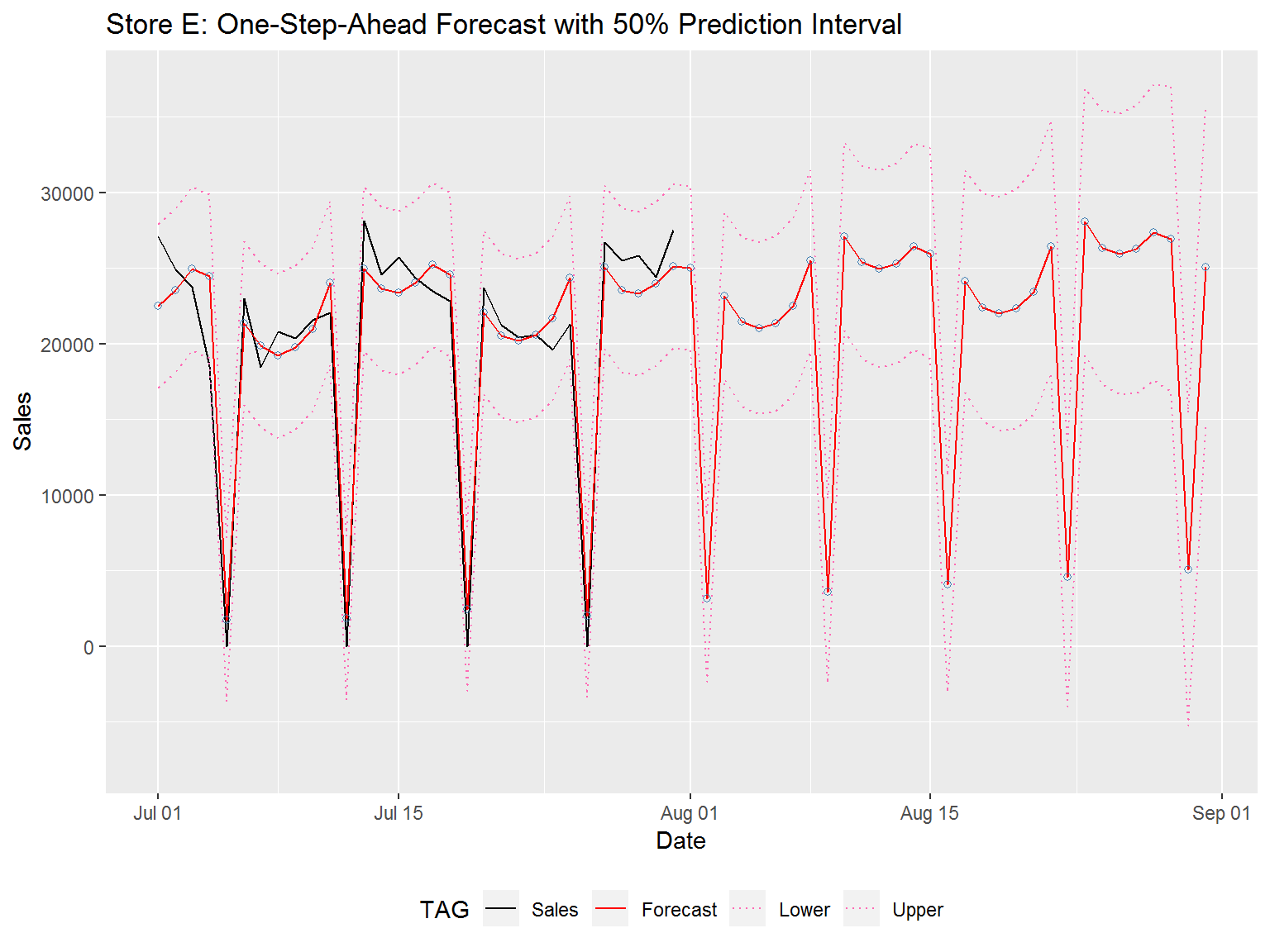
Note that our models do not understand that stores A, D and E are always closed on Sunday and hence should get 0 sales for this day. Asides from this flaw we see various trends for our stores. Store A has 0 sales on Sunday with weekday values being highest on Monday and then decreasing through Friday. Store D has similar behavior to store A. Store E on the other hand has high weekday values on Monday and Friday. Store B has the high sales spikes on Sundays. All stores tend to have weak sales figures between Tuesday and Thursday, though promotional events make a big difference and certainly help with the sales. We see this as weekdays with a promotional event have higher values than weekdays without a promotional event.
Two Year Monthly Forecasting
In this section we will do a two year forecast with monthly data. To get the monthly data we took, for each store, the average sales for that month based on the given data. We excluded days on which the store was closed or for which sales numbers were unknown. From this we use a Dynamic Linear Model (DLM) having local linear trend and monthly seasonality.
The ACF values we get below indicate that we have minimal correlation in the residuals from our model predictions. So there may be a better model, but this seems fairly good. As for the Q-Q plots, we will assume that our data is roughly normal. The big outliers in the Q-Q plot are likely due to the model needing a few iterations to fit to the data. We have not, in this case, removed those initial residuals from our model.
Below we include the one-step-ahead forecasts for our data. We can see that our predictions take around a year to fit the data, but afterwards are fairly good. This is a good argument for the forecasting ability of our models.

In addition to the graph above we include error estimates for our residuals based on the most recent 12 predictions. In particular, our Mean Absolute Error (MAE) is fairly small compared to the size of our sales values. Note that we did not use more months for our error analysis for two reasons. First, our earlier estimates are bad due to the model still trying to fit the data. Secondly, we will also consider a one year forecast based only on the first 19 months and we want to compare that forecast to these values.
| MAE | RMSE | MAPE | |
|---|---|---|---|
| Store A | 603.2547 | 736.0183 | 0.0311592 |
| Store B | 695.2972 | 904.2438 | 0.0337114 |
| Store C | 367.5026 | 433.4082 | 0.0204790 |
| Store D | 978.1973 | 1172.2721 | 0.0469504 |
| Store E | 650.4757 | 829.0892 | 0.0294282 |
We now include our two year forecasts. We can see below that we are forecasting a decrease in sales for store D and for store E we are forecasting an increase in sales. The other stores are more stable. This indicates that we may want to learn more about what is happening in store D and store E to prevent further sales loss on the one hand and learn how to mimic the success in sales revenue on the other.

We now fit our model to 19 Months worth of data instead of the full 31. This is allows use to make a one year prediction from which we can compare those results to the actual historical data without giving our model an unfair advantage. We see our one-step-ahead monthly predictions for the first 19 months below.

Here we can see ACF and Q-Q plots for our residuals.

Here we have visualizations for our one year forecasts.

Finally, we calculate error values based on the residuals for our 12 months of prediction. While not quite as good as our previous results, this seems fairly good since the model was not fit using the data and had to predict 12 months into the future with no extra guidance. We conclude that our two year forecast, which is based on the same type of model, is likely fairly good as well.
| MAE | RMSE | MAPE | |
|---|---|---|---|
| Store A | 857.1554 | 1026.7179 | 0.0435725 |
| Store B | 727.4460 | 909.6505 | 0.0358417 |
| Store C | 419.7701 | 507.0458 | 0.0233226 |
| Store D | 1070.5395 | 1384.7177 | 0.0504523 |
| Store E | 661.3382 | 863.5263 | 0.0295151 |
Conclusion
To conclude this project we believe that promotional events have a positive effect on sales revenue. Secondly we are interested in what store B does to get such high Sunday sales. Due to forecasted sales for Store D we believe an audit should be done on the store to figure out what is happening. We also note that Store D has the nearest competitor when looking at the original data. We would also like to know what store E is doing right to get a sharp increase in forecasted sales. Finally, we can see clear spikes in our monthly forecasts for the Winter and smaller spikes for the Summer. We should ensure sufficient employees are working during this time.