Introduction
Hello. In this post we will go over a variety of topics, however, the main focus will be classification. Our goal is to classify whether or not someone will default on a credit card payment in the next month based on certain variables. The data is from the UCI Machine Learning Repository and the reference to the data is at the bottom of this post. To determine whether someone defaults, we use a random forest to model the data. We will consider multiple models to determine which has the highest classification accuracy. As part of this process we try to use clustering. The idea for clustering came from the post “An Introduction to Clustering and different methods of clustering” which we reference below. The idea is to create new categories from the clustered data to see if we can enhance our classification accuracy. Finally, we compare some of our models by looking at receiver operating characteristic (ROC) curves and analyzing the results.
Below is a list of packages that were used.
# list of packages used
library(here)
library(randomForest)
library(ggplot2)
library(plotROC)
library(knitr)
Body
The first goal is to clean the data for use. We are given a variety of variables. Some variables are categorical and others are numerical. For the categorical variables Sex, Education and Marital Status we convert them into factors in R. We also have an ordinal categorical variable for History of Past Payment; we treat this variable as numerical since it is ordinal and the given values are already in the correct order. The rest of our covariate variables include information on the Amount of Credit Given, Age, Amount of Bill Statement, and Amount of Previous Payment.
# chunk to clean data
mydata_clean <- read.table(file = here::here("csv", "credit_card_clean.csv"), sep = ",", header = TRUE)

# put sex data into factor form with names
mydata_clean$SEX <- as.factor(mydata_clean$SEX)
levels(mydata_clean$SEX) <- c("M", "F")

# put education level into factor form with names
# note that data description list 4 types of education, but has 7  factors
# to deal with this we put the all the unlisted factor types into the other category
mydata_clean$EDUCATION <- as.factor(mydata_clean$EDUCATION)
levels(mydata_clean$EDUCATION)[levels(mydata_clean$EDUCATION) %in% c("0", "4", "5", "6")] <- "Other"
levels(mydata_clean$EDUCATION) <- c("other", "graduate_school", "university", "high_school")

# put marital status into factor form with names
# we combine the unexpected category into the other category
mydata_clean$MARRIAGE <- as.factor(mydata_clean$MARRIAGE)
levels(mydata_clean$MARRIAGE)[levels(mydata_clean$MARRIAGE) %in% c("0", "3")] <- "Other"
levels(mydata_clean$MARRIAGE) <- c("other", "married", "single")

# put default payment next month as factor DEFAULT with names
names(mydata_clean)[25] <- "DEFAULT"
mydata_clean$DEFAULT <- as.factor(mydata_clean$DEFAULT)
levels(mydata_clean$DEFAULT) <- c("NO", "YES")
Following the idea from the post we reference on clustering, we try using K means clustering with 2 to 8 clusters. We cluster based on the variables we left in numerical form. Our goal is to see if this clustering will give our model any meaningful enhancements to predictive accuracy. The next two chunks of code relate to our clustering.
# block for k-means clustering
set.seed(222)
cluster2 <- kmeans(mydata_clean[,c(2, 6:24)], centers = 2, nstart = 20)
cluster3 <- kmeans(mydata_clean[,c(2, 6:24)], centers = 3, nstart = 20)
cluster4 <- kmeans(mydata_clean[,c(2, 6:24)], centers = 4, nstart = 20)
cluster5 <- kmeans(mydata_clean[,c(2, 6:24)], centers = 5, nstart = 20)
cluster6 <- kmeans(mydata_clean[,c(2, 6:24)], centers = 6, nstart = 20)
cluster7 <- kmeans(mydata_clean[,c(2, 6:24)], centers = 7, nstart = 20)
cluster8 <- kmeans(mydata_clean[,c(2, 6:24)], centers = 8, nstart = 20)
# add cluster data as multiple categorical variables
mydata_clean$cluster2 <- as.factor(cluster2$cluster)
mydata_clean$cluster3 <- as.factor(cluster3$cluster)
mydata_clean$cluster4 <- as.factor(cluster4$cluster)
mydata_clean$cluster5 <- as.factor(cluster5$cluster)
mydata_clean$cluster6 <- as.factor(cluster6$cluster)
mydata_clean$cluster7 <- as.factor(cluster7$cluster)
mydata_clean$cluster8 <- as.factor(cluster8$cluster)Note that above we clustered on the entire dataset. Since it is reasonable to assume we can build a model and then perform clustering on old and new data to create a new set of clusters this should not be an issue. Alternatively we could try associating new data to pre-existing clusters. We now break half of our data into a testing set and the other half into a training set.
# chunk to split data into test and training sets
test_indices <- sample(1:nrow(mydata_clean), size = nrow(mydata_clean)/2)
test_data <- mydata_clean[test_indices,]
train_data <- mydata_clean[-test_indices,]
Now that we have training and testing datasets we fit our training data to various models to predict whether a person defaults on their credit card payments. Since our clusters were fit to the numerical data we first consider models which are fit only based on Sex, Education, and Marriage Status. These simple models also are fit based on the clusters. We are curious to see if the cluster data can capture the information from the numerical covariates. As a baseline we have 1 cluster (the default) and go all the way up to 8 clusters. In addition to our simple models, we also try models which contain all the covariates along with data for 1 to 8 clusters (1 being the default).
# chunk to compute multiple random forests
# simplified forest
forest_simple1 <- randomForest(DEFAULT ~ SEX + EDUCATION + MARRIAGE, data = train_data)
forest_simple2 <- randomForest(DEFAULT ~ SEX + EDUCATION + MARRIAGE + cluster2, data = train_data)
forest_simple3 <- randomForest(DEFAULT ~ SEX + EDUCATION + MARRIAGE + cluster3, data = train_data)
forest_simple4 <- randomForest(DEFAULT ~ SEX + EDUCATION + MARRIAGE + cluster4, data = train_data)
forest_simple5 <- randomForest(DEFAULT ~ SEX + EDUCATION + MARRIAGE + cluster5, data = train_data)
forest_simple6 <- randomForest(DEFAULT ~ SEX + EDUCATION + MARRIAGE + cluster6, data = train_data)
forest_simple7 <- randomForest(DEFAULT ~ SEX + EDUCATION + MARRIAGE + cluster7, data = train_data)
forest_simple8 <- randomForest(DEFAULT ~ SEX + EDUCATION + MARRIAGE + cluster8, data = train_data)

# full forest
forest_full1 <- randomForest(DEFAULT ~., data = train_data[, c(1:25)])
forest_full2 <- randomForest(DEFAULT ~., data = train_data[, c(1:25, 26)])
forest_full3 <- randomForest(DEFAULT ~., data = train_data[, c(1:25, 27)])
forest_full4 <- randomForest(DEFAULT ~., data = train_data[, c(1:25, 28)])
forest_full5 <- randomForest(DEFAULT ~., data = train_data[, c(1:25, 29)])
forest_full6 <- randomForest(DEFAULT ~., data = train_data[, c(1:25, 30)])
forest_full7 <- randomForest(DEFAULT ~., data = train_data[, c(1:25, 31)])
forest_full8 <- randomForest(DEFAULT ~., data = train_data[, c(1:25, 32)])
We now consider the classification accuracy of our models. We plot the data below based on whether we have a simple or full model as described above. We additionally include the number of clusters.
# chunk to look at classification accuracy
forest_simple1_predict <- predict(forest_simple1, newdata = test_data[, -25])
a1 <- mean(forest_simple1_predict == test_data[,25]) # classification accuracy
forest_simple2_predict <- predict(forest_simple2, newdata = test_data[, -25])
a2 <- mean(forest_simple2_predict == test_data[,25]) # classification accuracy
forest_simple3_predict <- predict(forest_simple3, newdata = test_data[, -25])
a3 <- mean(forest_simple3_predict == test_data[,25]) # classification accuracy
forest_simple4_predict <- predict(forest_simple4, newdata = test_data[, -25])
a4 <- mean(forest_simple4_predict == test_data[,25]) # classification accuracy
forest_simple5_predict <- predict(forest_simple5, newdata = test_data[, -25])
a5 <- mean(forest_simple5_predict == test_data[,25]) # classification accuracy
forest_simple6_predict <- predict(forest_simple6, newdata = test_data[, -25])
a6 <- mean(forest_simple6_predict == test_data[,25]) # classification accuracy
forest_simple7_predict <- predict(forest_simple7, newdata = test_data[, -25])
a7 <- mean(forest_simple7_predict == test_data[,25]) # classification accuracy
forest_simple8_predict <- predict(forest_simple8, newdata = test_data[, -25])
a8 <- mean(forest_simple8_predict == test_data[,25]) # classification accuracy

forest_full1_predict <- predict(forest_full1, newdata = test_data[, -25])
b1 <- mean(forest_full1_predict == test_data[,25]) # classification accuracy
forest_full2_predict <- predict(forest_full2, newdata = test_data[, -25])
b2 <- mean(forest_full2_predict == test_data[,25]) # classification accuracy
forest_full3_predict <- predict(forest_full3, newdata = test_data[, -25])
b3 <- mean(forest_full3_predict == test_data[,25]) # classification accuracy
forest_full4_predict <- predict(forest_full4, newdata = test_data[, -25])
b4 <- mean(forest_full4_predict == test_data[,25]) # classification accuracy
forest_full5_predict <- predict(forest_full5, newdata = test_data[, -25])
b5 <- mean(forest_full5_predict == test_data[,25]) # classification accuracy
forest_full6_predict <- predict(forest_full6, newdata = test_data[, -25])
b6 <- mean(forest_full6_predict == test_data[,25]) # classification accuracy
forest_full7_predict <- predict(forest_full7, newdata = test_data[, -25])
b7 <- mean(forest_full7_predict == test_data[,25]) # classification accuracy
forest_full8_predict <- predict(forest_full8, newdata = test_data[, -25])
b8 <- mean(forest_full8_predict == test_data[,25]) # classification accuracy

df <- data.frame(Accuracy = c(a1,a2,a3,a4,a5,a6,a7,a8,b1,b2,b3,b4,b5,b6,b7,b8),
                 Clusters = c(1:8,1:8), Type = c(rep("Simple", 8), rep("Full", 8)))

ggplot(df, aes(x = Clusters, y = Accuracy, col = Type)) +
  geom_line() + geom_point() + ggtitle("Classification Accuracy of Models")
The graph above indicates two things. Firstly, the full model is better at prediction. Secondly, we can see that, in this case, the number of clusters does not enhance prediction and even appears to reduce classification accuracy. Based on these results we will only consider the simple and full models without clustering (that is having a single default cluster).
For the simple model we have a classification table below. What we can see is that the model always predicts that there is no default. This is a model we could come up with without doing any calculations.
# chunk for classification tables
sfp_response <- predict(forest_simple1, newdata = test_data[, -25], type = "response")
correct_yes <- sum(sfp_response == "YES" & test_data[,"DEFAULT"] == "YES")
correct_no <- sum(sfp_response == "NO" & test_data[,"DEFAULT"] == "NO")
wrong_yes <- sum(sfp_response == "YES" & test_data[,"DEFAULT"] == "NO")
wrong_no <- sum(sfp_response == "NO" & test_data[,"DEFAULT"] == "YES")

classvector_simple <- c(correct_yes, wrong_no, wrong_yes, correct_no)
classtable_simple <- matrix(data = classvector_simple, nrow = 2, ncol = 2, byrow = TRUE)
rownames(classtable_simple) <- c("Actual Default", "Actual No Default")
colnames(classtable_simple) <- c("Predict Default", "Predict No Default")

kable(classtable_simple, row.names = TRUE)| Predict Default | Predict No Default | |
|---|---|---|
| Actual Default | 0 | 3310 |
| Actual No Default | 0 | 11690 |
# sensitivity and specificity
sensitivity_simple <- (correct_yes)/ (correct_yes + wrong_no)
specificity_simple <- (correct_no)/ (correct_no + wrong_yes)
Based on our results our simple model has no ability to predict a default. We see that our sensitivity is 0 and our specificity is 1. Overall, this is not a very useful model. As we saw in our graph, our full model has higher classification accuracy. Below we include the associated classification table for our full model.
# chunk for classification tables
ffp_response <- predict(forest_full1, newdata = test_data[, -25], type = "response")
correct_yes <- sum(ffp_response == "YES" & test_data[,"DEFAULT"] == "YES")
correct_no <- sum(ffp_response == "NO" & test_data[,"DEFAULT"] == "NO")
wrong_yes <- sum(ffp_response == "YES" & test_data[,"DEFAULT"] == "NO")
wrong_no <- sum(ffp_response == "NO" & test_data[,"DEFAULT"] == "YES")

classvector_full <- c(correct_yes, wrong_no, wrong_yes, correct_no)
classtable_full <- matrix(data = classvector_full, nrow = 2, ncol = 2, byrow = TRUE)
rownames(classtable_full) <- c("Actual Default", "Actual No Default")
colnames(classtable_full) <- c("Predict Default", "Predict No Default")

kable(classtable_full, row.names = TRUE)| Predict Default | Predict No Default | |
|---|---|---|
| Actual Default | 1171 | 2139 |
| Actual No Default | 581 | 11109 |
# sensitivity and specificity
sensitivity_full <- (correct_yes)/ (correct_yes + wrong_no)
specificity_full <- (correct_no)/ (correct_no + wrong_yes)
Sensitivity for our full model is 0.3537764 while specificity for our full model is 0.9502994. So we can see that for a small loss in correctly predicting someone will not default on credit card payments we are now much better able to predict a default in credit card payments. Moreover, our overall classification accuracy is better in the full model.
Conclusion and ROC Curves
# block for ROC curves
sfp <- predict(forest_simple1, newdata = test_data[, -25], type = "prob")
ffp <- predict(forest_full1, newdata = test_data[, -25], type = "prob")
ggplot(test_data, aes(d = DEFAULT, m = sfp[,2])) +
  geom_roc(labels = FALSE) + coord_fixed() +
  xlab("1 - Specificity") + ylab("Sensitivity") +
  ggtitle("ROC Curve for Simple Model")
## Warning in verify_d(data$d): D not labeled 0/1, assuming NO = 0 and YES =
## 1!
point_full <- data.frame(x = sensitivity_full, y = 1 - specificity_full)

ggplot(test_data, aes(d = test_data$DEFAULT, m = ffp[,2])) +
  geom_roc(labels = FALSE) + coord_fixed() +

  xlab("1 - Specificity") + ylab("Sensitivity") +
  ggtitle("ROC Curve for Full Model")
## Warning in verify_d(data$d): D not labeled 0/1, assuming NO = 0 and YES =
## 1!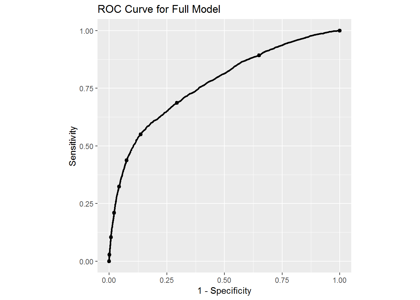
From the simple model we see that the ROC curve is a straight line indicating that we get the same accuracy in our model simply by making an educated guess based on the proportion of defaults. So this simple model is not very useful. In the case of the full model we see a more reasonable ROC curve. Indeed, with the full model we could adjust how predictions are done to perhaps further increase sensitivity by decreasing specificity. This could be useful if we are more concerned with determining who will default rather than those who will not default. Changing the value on the ROC curve could affect overall classification accuracy, so if we are mostly concerned with that we would have to look a different metric. We will leave those considerations for the future.
References:
For data: https://archive.ics.uci.edu/ml/datasets/default+of+credit+card+clients#
For article: An Introduction to Clustering and different methods of clustering https://www.analyticsvidhya.com/blog/2016/11/an-introduction-to-clustering-and-different-methods-of-clustering/