Introduction
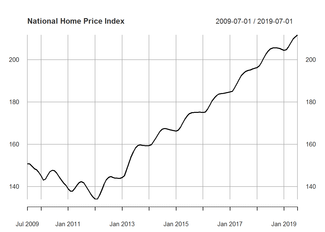
In this post we focus on time series and forecasting. We will use the dlm package written by Dr. Giovanni Petris. The dlm package creates dynamic linear models that we use in forecasting. For our data, we will use the S&P/Case-Shiller U.S. National Home Price Index which we reference at the end of this post. We include our R code in the appendix, but will not include it in the main body of this post for readability. We begin by examining our time series data. Note that Jan 2000 is used for index value 100. A plot of the data is included below.

As we can see, the index value tends to increase. There is, however, a significant decrease between the years 2007 and 2012. Notice that there is no significant seasonal behavior at first, but this appears to change around the year 2009. One of the major goals of this post will be to examine how the change from non-seasonal to seasonal behavior affects our predictions.
Section 1
Our first goal is to create models to fit the data. Since we are using the dlm package, this means we need to create model skeletons. We can create the model skeletons to take into account properties such as linearity and seasonality. Once we have our model skeletons, we must fit our models to the data. This determines our model parameters and is done through the dlmMLE function.
We have some idea how the data behaves based on the graph. In our case, it is unclear whether seasonality is important in our model. So we will create four models. Our models are the local level (LL), local linear trend (LLT), local level with seasonality (LLS), and local linear trend with seasonality (LLTS). Note that we will only consider monthly seasonality.
Once we have our fitted models, we would like to determine which model fits the data best. Methods for model selection include: graphical comparison, model selection criterion, and minimizing prediction error. For this first section, we will focus on just model selection criterion and minimizing prediction error.
For model selection criterion, we will use the Akaike information criterion (AIC) and the Bayesian information criterion (BIC). The model with the lowest value is considered the best. Based on the following table, our linear trend model has both the lowest AIC and the lowest BIC while the local linear trend with seasonality has the second lowest AIC and BIC. Based on this result we should conclude that the local linear trend model is superior.
##                                AIC       BIC
## Local Level (LL)          433.1212  441.0586
## Local Linear Trend (LLT) -253.7366 -241.8305
## (LL) with Seasonality     551.9132  563.8193
## (LLT) with Seasonality   -234.6613 -218.7865
Since a major objective of time series is forecasting, we also consider prediction error based on one-step-ahead predictions. We measure error using the following methods: mean absolute error (MAE), root mean square error (RMSE), and mean absolute percentage error (MAPE). Based on results in the table below, the best model is clearly the local linear trend model which has the lowest or near lowest error of each type. It is worth noting that the models with seasonality tend to have the highest or close to the highest errors. This will be examined more in the next section.
## MAE RMSE MAPE
## Local Level (LL) 1.32649 3.58770 0.01124
## Local Linear Trend (LLT) 0.72424 3.66798 0.00734
## (LL) with Seasonality 2.53157 5.77651 0.02427
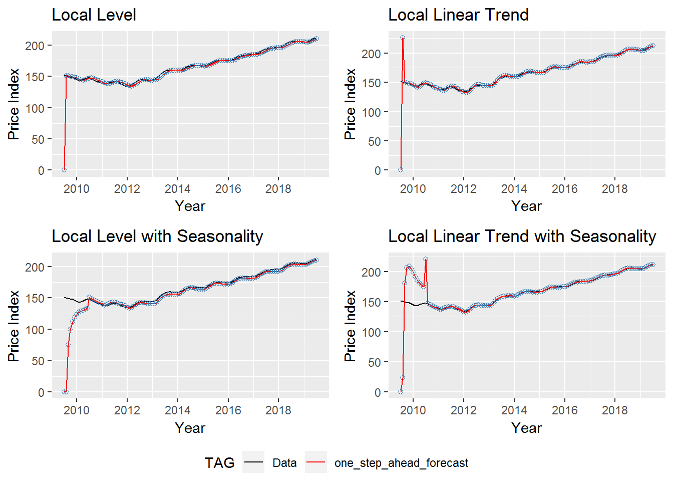
## (LLT) with Seasonality 1.23396 5.53226 0.01582Based on both model selection criterion and looking at the prediction error we conclude, for now, that the local linear trend model is the best. Notice below how well our one-step-ahead predictions follow our model.

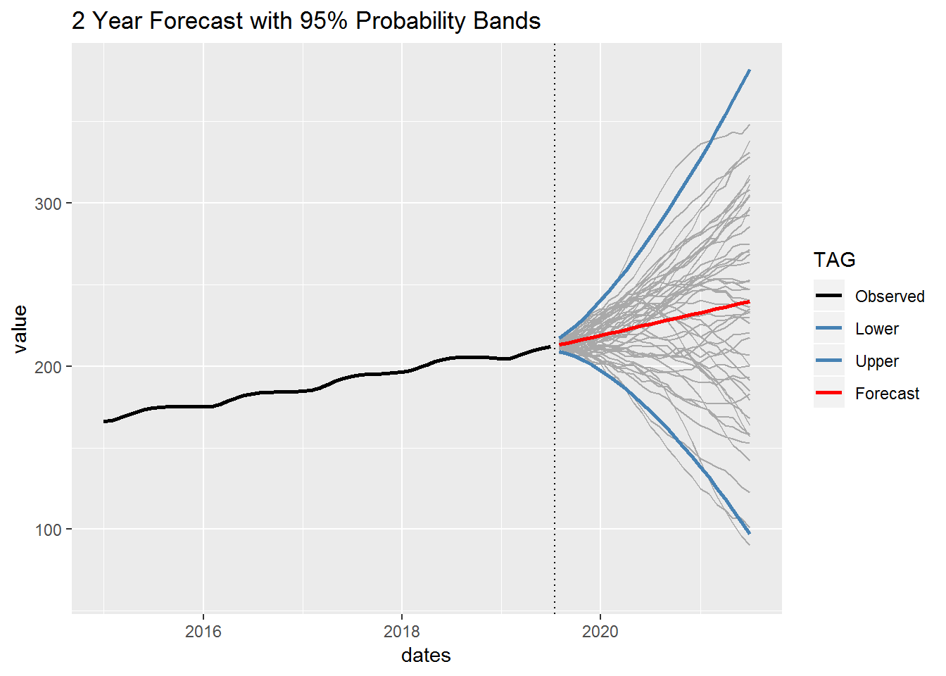
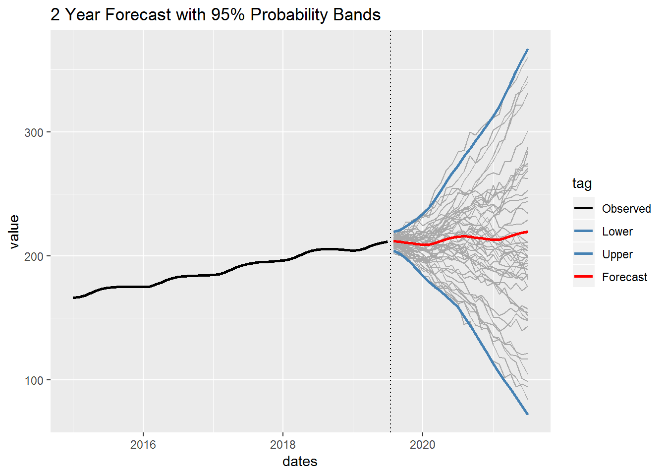
To conclude this section we include a 2 year forecast based on our chosen model. For this, we focus the most recent part of our time series. We include \(95\%\) probability bands and the forecast. We also have fifty small lines representing randomly generated outcomes based on our model. Finally, notice that our forecast is simply a straight line with a positive slope. This is due to our choice of the local linear trend model. So if we run out of data our forecast will end up being a straight line with this model. This is in contrast to one-step-ahead forecasts which are constantly updated based on the data.
Section 2
In the previous section, we concluded that the local linear trend model was the best. For the entire dataset this seems reasonable, but for the most recent values in time we see what appear to be monthly fluctuations. So we will fit the same models on just the most recent 10 years of data where the seasonal fluctuations begin. Below is a graph of the data we are now considering.
We fit the data to the model skeletons we used in Section 1. We consider model selection criterion and one-step-ahead prediction error for the models. Our results are shown below.
##                              AIC       BIC
## Local Level            195.68498 201.27656
## Local Linear Trend      48.84603  57.23340
## (LL) with Seasonality  307.35830 315.74567
## (LLT) with Seasonality  95.41550 106.59866
## MAE RMSE MAPE
## Local Level 2.74433 13.83021 0.01750
## Local Linear Trend 2.72170 15.36402 0.01775
## (LL) with Seasonality 6.82604 21.80344 0.04432
## (LLT) with Seasonality 7.04695 23.32045 0.04735The above results are somewhat surprising. Model selection criterion seems reasonable enough with the local linear trend model beating the local linear trend with seasonality model. Perhaps having fewer parameters is good for model efficiency. What seems strange, however, is that the prediction error for the models with seasonality is fairly bad compared to the other models. Rather than ignore this, we will look at the graphs for each model. Below we look at the one-step-ahead forecasts for each of our models.
The first thing we notice is that each model starts with an initial value of zero. So there is a large jump needed to correctly estimate the trend. The local level and local linear trend models adjust very quickly, but the models with seasonality take about a year to adjust to the correct value. We will remove the first two years of residuals to ensure the model has enough time to adjust to the data. This is reasonable since it takes the seasonal models around a year to adjust to the data. We also do not want to estimate our error based on early predictions that clearly do not represent the accuracy of our models as a whole. We now recompute our error estimates by removing the earliest 2 years of residual data.
## MAE RMSE MAPE
## Local Level 1.48740 1.89159 0.00886
## Local Linear Trend 0.82279 1.02971 0.00500
## (LL) with Seasonality 2.27176 2.46266 0.01335
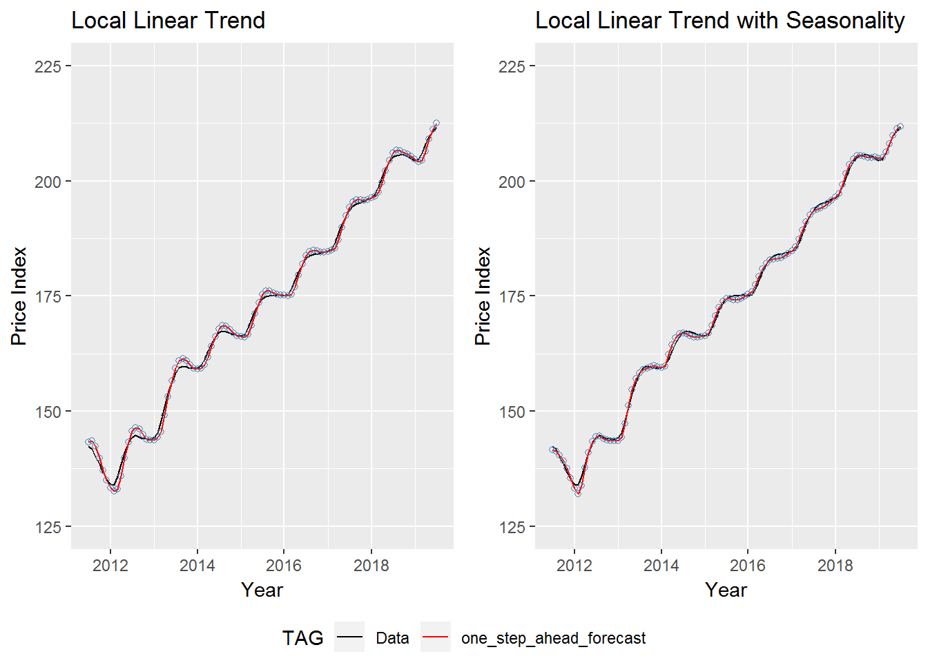
## (LLT) with Seasonality 0.50538 0.62407 0.00305As we can see above, removing the first couple years of residuals from our error calculation indicates that the local linear trend with seasonality model is the best at one-step-ahead prediction. Below we will compare both local linear trend models graphically against the actual data. We only consider the years our new error estimates are based on. While both models are good, we can see that the local linear trend with seasonality model fits the data just a little better.
We conclude this section with a 2 year forecast using the local linear trend with seasonality model. In this case our prediction has a clear linear trend, but also takes into account seasonality.
Conclusion
Looking at just error estimates or model selection criterion can be useful, but it is beneficial to visualize the data as well. We saw in Section 2 that the error estimates hinted at something odd happening, but we may not have suspected anything without our initial observation of a possible seasonal trend. We could see even more when we graphed our predictions. Based on these observations, it would be appropriate to go back to Section 1 and re-evaluate our prediction errors after giving the models a little more time to adjust to the data.
Note that we only did in-sample error estimates. We could have withheld some of our most recent data and compared a 1 or 2 year forecast against actual historical results. This could potentially end up with a different model being selected.
Ultimately, I hope this blog shows how the dlm package is able to utilize time series data for effective one-step-ahead predictions and also in longer term forecasting.
Reference for data:
S&P Dow Jones Indices LLC, S&P/Case-Shiller U.S. National Home Price Index [CSUSHPINSA], retrieved from FRED, Federal Reserve Bank of St. Louis; https://fred.stlouisfed.org/series/CSUSHPINSA, October 1, 2019.
Appendix:
This section includes all of the code used in the R Markdown chunks in this document. To reproduce the result you will need the data found at https://fred.stlouisfed.org/series/CSUSHPINSA and use the data from 1987-01-01 to 2019-07-01. Instead of setting up a project and using the here package the data can be directly referenced.
library(forecast)
library(dlm)
library(here)
library(xts)
library(ggplot2)
library(reshape2) # for melting lists or dataframes
library(ggpubr) # used instead of gridExtra


# read and store dataset for use
mydata <- read.table(here("csv", "National_Home_Price_Index.csv"), header = TRUE, sep = ",")
# convert dataframe into class xts
time <- as.POSIXct(mydata[,1])
nhpi <- xts(mydata[,2], time)
plot(nhpi, main = "National Home Price Index")


# local level model
mod_nhpi_ll <- dlmModPoly(1) # model 'skeleton'
build_nhpi_ll <- function(u) { #function to pass to dlmMLE
u <- exp(u)
mod_nhpi_ll$V[] <- u[1]
mod_nhpi_ll$W[] <- u[2]
mod_nhpi_ll
}
fit_nhpi_ll <- dlmMLE(nhpi, c(10, 1), build_nhpi_ll)
fit_nhpi_ll$conv # result of 0 indicates convergence (must be 0)
fit_nhpi_ll$value

# local linear trend model
mod_nhpi_llt <- dlmModPoly(2) # model 'skeleton'
build_nhpi_llt <- function(u) { #function to pass to dlmMLE
u <- exp(u)
mod_nhpi_llt$V[] <- u[1]
diag(mod_nhpi_llt$W)[1:2]<- u[2:3]
mod_nhpi_llt
}
fit_nhpi_llt <- dlmMLE(nhpi, c(2, 1, 1), build_nhpi_llt)
fit_nhpi_llt$conv # result of 0 indicates convergence
fit_nhpi_llt$value

# local level with seasonality model
mod_nhpi_lls <- dlmModPoly(1) + dlmModSeas(12) # model 'skeleton'
build_nhpi_lls <- function(u) { #function to pass to dlmMLE
u <- exp(u)
mod_nhpi_lls$V[] <- u[1]
diag(mod_nhpi_lls$W)[1:2] <- u[2:3]
mod_nhpi_lls
}
fit_nhpi_lls <- dlmMLE(nhpi, rep(0,3), build_nhpi_lls)
fit_nhpi_lls$conv # result of 0 indicates convergence
fit_nhpi_lls$value

# local linear trend with seasonality model
mod_nhpi_llts <- dlmModPoly(2) + dlmModSeas(12) # model 'skeleton'
build_nhpi_llts <- function(u) { #function to pass to dlmMLE
u <- exp(u)
mod_nhpi_llts$V[] <- u[1]
diag(mod_nhpi_llts$W)[1:3] <- u[2:4]
mod_nhpi_llts
}
fit_nhpi_llts <- dlmMLE(nhpi, c(2, 1, 0, 2), build_nhpi_llts)
fit_nhpi_llts$conv # result of 0 indicates convergence
fit_nhpi_llts$value


selection <- matrix(c(
2 * fit_nhpi_ll$value + 2 * length(fit_nhpi_ll$par),
2 * fit_nhpi_llt$value + 2 * length(fit_nhpi_llt$par),
2 * fit_nhpi_lls$value + 2 * length(fit_nhpi_lls$par),
2 * fit_nhpi_llts$value + 2 * length(fit_nhpi_llts$par),
2 * fit_nhpi_ll$value + log(length(nhpi)) * length(fit_nhpi_ll$par),
2 * fit_nhpi_llt$value + log(length(nhpi)) * length(fit_nhpi_llt$par),
2 * fit_nhpi_lls$value + log(length(nhpi)) * length(fit_nhpi_lls$par),
2 * fit_nhpi_llts$value + log(length(nhpi)) * length(fit_nhpi_llts$par))
,ncol=2, byrow=FALSE)
colnames(selection) <- c("AIC","BIC")
rownames(selection) <- c("Local Level (LL)","Local Linear Trend (LLT)",
                         "(LL) with Seasonality","(LLT) with Seasonality")
(selection <- as.table(selection))


prediction <- matrix(c(
    mean(abs(residuals(dlmFilter(nhpi, mod_nhpi_ll), type = "raw", sd = FALSE))),
    mean(abs(residuals(dlmFilter(nhpi, mod_nhpi_llt), type = "raw", sd = FALSE))),
    mean(abs(residuals(dlmFilter(nhpi, mod_nhpi_lls), type = "raw", sd = FALSE))),
    mean(abs(residuals(dlmFilter(nhpi, mod_nhpi_llts), type = "raw", sd = FALSE))),
    sqrt(mean(residuals(dlmFilter(nhpi, mod_nhpi_ll), type = "raw", sd = FALSE)^2)),
    sqrt(mean(residuals(dlmFilter(nhpi, mod_nhpi_llt), type = "raw", sd = FALSE)^2)),
    sqrt(mean(residuals(dlmFilter(nhpi, mod_nhpi_lls), type = "raw", sd = FALSE)^2)),
    sqrt(mean(residuals(dlmFilter(nhpi, mod_nhpi_llts), type = "raw", sd = FALSE)^2)),
    mean(abs(residuals(dlmFilter(nhpi, mod_nhpi_ll), type = "raw", sd = FALSE)) / nhpi),
    mean(abs(residuals(dlmFilter(nhpi, mod_nhpi_llt), type = "raw", sd = FALSE)) / nhpi),
    mean(abs(residuals(dlmFilter(nhpi, mod_nhpi_lls), type = "raw", sd = FALSE)) / nhpi),
    mean(abs(residuals(dlmFilter(nhpi, mod_nhpi_llts), type = "raw", sd = FALSE)) / nhpi))
  ,ncol=3, byrow=FALSE)
colnames(prediction) <- c("MAE","RMSE", "MAPE")
rownames(prediction) <- c("Local Level (LL)","Local Linear Trend (LLT)",
                         "(LL) with Seasonality","(LLT) with Seasonality")
(prediction <- as.table(round(prediction, 5)))


# Local Linear Trend
filt_nhpi_llt <- dlmFilter(nhpi, mod_nhpi_llt)

df1 <- data.frame(time = index(nhpi), value = nhpi[,1], TAG = "Data")
df2 <- data.frame(time = index(filt_nhpi_llt$f), value = filt_nhpi_llt$f[,1], TAG = "one_step_ahead_forecast")
df3 <- data.frame(time = index(filt_nhpi_llt$f), value = filt_nhpi_llt$f[,1], TAG = "Points")
df <- rbind(df1, df2)

ggplot() +
  geom_line(data = df, aes(x = time, y = value, col = TAG)) +
  scale_colour_manual(values=c(Data='black', one_step_ahead_forecast='red')) +
  geom_point(data = df3, aes(x = time, y = value), col = "steelblue", shape = 1) +
  xlab("Year") +
  ylab("Price Index") +
  theme(legend.position = "bottom") +
  ggtitle("Local Linear Trend One-Step-Ahead-Forecast")


# k-steps ahead forecast
set.seed(122)
future_nhpi <- dlmForecast(filt_nhpi_llt, nAhead = 24, sampleNew = 50)

df1 <- data.frame(time = index(nhpi), value = nhpi[,1], TAG = "Observed")

dates <- seq(as.Date("2019-08-02"), length=24, by="months") # We added a day
dates <- round(as.POSIXct(dates), units = "months") # as.POSIXCT seems to lower the date by 1 day.

df2 <- data.frame(time = dates, value = future_nhpi$f + sqrt(unlist(future_nhpi$Q)) * qnorm(0.025), TAG = "Lower")
df3 <- data.frame(time = dates, value = future_nhpi$f + sqrt(unlist(future_nhpi$Q)) * qnorm(0.975), TAG = "Upper")
df4 <- data.frame(time = dates, value = future_nhpi$f, TAG = "Forecast")
df <- rbind(df1, df2, df3, df4)

melted_df <- melt(future_nhpi$newObs) # using reshape2 package for melt
long_dates <- rep(dates,50)
melted_df$dates <- as.POSIXct(long_dates)

suppressWarnings(print(
  ggplot() +
    geom_line(data = melted_df, aes(x = dates, y = value, group = L1), linetype = "solid", color = "darkgrey") +
    geom_vline(xintercept = mean(c(end(nhpi), as.POSIXct("2019-08-01"))), linetype = "dotted") +
    geom_line(data = df, aes(time, value, col = TAG), lwd = 1) +
    xlim(as.POSIXct(c("2015-01-01", "2021-07-01"))) +
    scale_colour_manual(values=c(Observed='black', Forecast='red', Upper='steelblue', Lower='steelblue')) +
    ggtitle("2 Year Forecast with 95% Probability Bands")
))


old_nhpi <- nhpi # store original time series for future use
nhpi <- nhpi[271:391,] # use the most recent 10 years of data
plot(nhpi, main = "National Home Price Index")


# local level
mod_nhpi_ll <- dlmModPoly(1) # model 'skeleton'
build_nhpi_ll <- function(u) {
u <- exp(u)
mod_nhpi_ll$V[] <- u[1]
mod_nhpi_ll$W[] <- u[2]
mod_nhpi_ll
}
fit_nhpi_ll <- dlmMLE(nhpi, c(1, 1), build_nhpi_ll)
fit_nhpi_ll$conv # result of 0 indicates convergence
fit_nhpi_ll$value

# local linear trend
mod_nhpi_llt <- dlmModPoly(2) # model 'skeleton'
build_nhpi_llt <- function(u) {
u <- exp(u)
mod_nhpi_llt$V[] <- u[1]
diag(mod_nhpi_llt$W)[1:2]<- u[2:3]
mod_nhpi_llt
}
fit_nhpi_llt <- dlmMLE(nhpi, c(2, 1, 1), build_nhpi_llt)
fit_nhpi_llt$conv
fit_nhpi_llt$value

# local level with seasonality
mod_nhpi_lls <- dlmModPoly(1) + dlmModSeas(12) # model 'skeleton'
build_nhpi_lls <- function(u) {
u <- exp(u)
mod_nhpi_lls$V[] <- u[1]
diag(mod_nhpi_lls$W)[1:2] <- u[2:3]
mod_nhpi_lls
}
fit_nhpi_lls <- dlmMLE(nhpi, c(2, 1, 1), build_nhpi_lls)
fit_nhpi_lls$conv
fit_nhpi_lls$value

# local linear trend with seasonality
mod_nhpi_llts <- dlmModPoly(2) + dlmModSeas(12) # model 'skeleton'
build_nhpi_llts <- function(u) {
u <- exp(u)
mod_nhpi_llts$V[] <- u[1]
diag(mod_nhpi_llts$W)[1:3] <- u[2:4]
mod_nhpi_llts
}
fit_nhpi_llts <- dlmMLE(nhpi, c(1, -2, 0, -1), build_nhpi_llts)
fit_nhpi_llts$conv
fit_nhpi_llts$value


selection <- matrix(c(
2 * fit_nhpi_ll$value + 2 * length(fit_nhpi_ll$par),
2 * fit_nhpi_llt$value + 2 * length(fit_nhpi_llt$par),
2 * fit_nhpi_lls$value + 2 * length(fit_nhpi_lls$par),
2 * fit_nhpi_llts$value + 2 * length(fit_nhpi_llts$par),
2 * fit_nhpi_ll$value + log(length(nhpi)) * length(fit_nhpi_ll$par),
2 * fit_nhpi_llt$value + log(length(nhpi)) * length(fit_nhpi_llt$par),
2 * fit_nhpi_lls$value + log(length(nhpi)) * length(fit_nhpi_lls$par),
2 * fit_nhpi_llts$value + log(length(nhpi)) * length(fit_nhpi_llts$par))
,ncol=2, byrow=FALSE)
colnames(selection) <- c("AIC","BIC")
rownames(selection) <- c("Local Level","Local Linear Trend",
                         "(LL) with Seasonality","(LLT) with Seasonality")
(selection <- as.table(selection))


prediction <- matrix(c(
    mean(abs(residuals(dlmFilter(nhpi, mod_nhpi_ll), type = "raw", sd = FALSE))),
    mean(abs(residuals(dlmFilter(nhpi, mod_nhpi_llt), type = "raw", sd = FALSE))),
    mean(abs(residuals(dlmFilter(nhpi, mod_nhpi_lls), type = "raw", sd = FALSE))),
    mean(abs(residuals(dlmFilter(nhpi, mod_nhpi_llts), type = "raw", sd = FALSE))),
    sqrt(mean(residuals(dlmFilter(nhpi, mod_nhpi_ll), type = "raw", sd = FALSE)^2)),
    sqrt(mean(residuals(dlmFilter(nhpi, mod_nhpi_llt), type = "raw", sd = FALSE)^2)),
    sqrt(mean(residuals(dlmFilter(nhpi, mod_nhpi_lls), type = "raw", sd = FALSE)^2)),
    sqrt(mean(residuals(dlmFilter(nhpi, mod_nhpi_llts), type = "raw", sd = FALSE)^2)),
    mean(abs(residuals(dlmFilter(nhpi, mod_nhpi_ll), type = "raw", sd = FALSE)) / nhpi),
    mean(abs(residuals(dlmFilter(nhpi, mod_nhpi_llt), type = "raw", sd = FALSE)) / nhpi),
    mean(abs(residuals(dlmFilter(nhpi, mod_nhpi_lls), type = "raw", sd = FALSE)) / nhpi),
    mean(abs(residuals(dlmFilter(nhpi, mod_nhpi_llts), type = "raw", sd = FALSE)) / nhpi))
  ,ncol=3, byrow=FALSE)
colnames(prediction) <- c("MAE","RMSE", "MAPE")
rownames(prediction) <- c("Local Level","Local Linear Trend",
                         "(LL) with Seasonality","(LLT) with Seasonality")
(prediction <- as.table(round(prediction, 5)))


# filtered models
filt_nhpi_ll <- dlmFilter(nhpi, mod_nhpi_ll)
filt_nhpi_llt <- dlmFilter(nhpi, mod_nhpi_llt)
filt_nhpi_lls <- dlmFilter(nhpi, mod_nhpi_lls)
filt_nhpi_llts <- dlmFilter(nhpi, mod_nhpi_llts)


# local level plot
df1 <- data.frame(time = index(nhpi), value = nhpi[,1], TAG = "Data")
df2 <- data.frame(time = index(filt_nhpi_ll$f), value = filt_nhpi_ll$f[,1], TAG = "one_step_ahead_forecast")
df3 <- data.frame(time = index(filt_nhpi_ll$f), value = filt_nhpi_ll$f[,1], TAG = "Points")
df <- rbind(df1, df2)

plot1 <- ggplot() +
  geom_line(data = df, aes(x = time, y = value, col = TAG)) +
  scale_colour_manual(values=c(Data='black', one_step_ahead_forecast='red')) +
  geom_point(data = df3, aes(x = time, y = value), col = "steelblue", shape = 1) +
  xlab("Year") +
  ylab("Price Index") +
  ggtitle("Local Level")

# local linear trend plot
df1 <- data.frame(time = index(nhpi), value = nhpi[,1], TAG = "Data")
df2 <- data.frame(time = index(filt_nhpi_llt$f), value = filt_nhpi_llt$f[,1], TAG = "one_step_ahead_forecast")
df3 <- data.frame(time = index(filt_nhpi_llt$f), value = filt_nhpi_llt$f[,1], TAG = "Points")
df <- rbind(df1, df2)

plot2 <- ggplot() +
  geom_line(data = df, aes(x = time, y = value, col = TAG)) +
  scale_colour_manual(values=c(Data='black', one_step_ahead_forecast='red')) +
  geom_point(data = df3, aes(x = time, y = value), col = "steelblue", shape = 1) +
  xlab("Year") +
  ylab("Price Index") +
  ggtitle("Local Linear Trend")

# local level with seasonality plot
df1 <- data.frame(time = index(nhpi), value = nhpi[,1], TAG = "Data")
df2 <- data.frame(time = index(filt_nhpi_lls$f), value = filt_nhpi_lls$f[,1], TAG = "one_step_ahead_forecast")
df3 <- data.frame(time = index(filt_nhpi_lls$f), value = filt_nhpi_lls$f[,1], TAG = "Points")
df <- rbind(df1, df2)

plot3 <- ggplot() +
  geom_line(data = df, aes(x = time, y = value, col = TAG)) +
  scale_colour_manual(values=c(Data='black', one_step_ahead_forecast='red')) +
  geom_point(data = df3, aes(x = time, y = value), col = "steelblue", shape = 1) +
  xlab("Year") +
  ylab("Price Index") +
  ggtitle("Local Level with Seasonality")

# local linear trend with seasonality plot
df1 <- data.frame(time = index(nhpi), value = nhpi[,1], TAG = "Data")
df2 <- data.frame(time = index(filt_nhpi_llts$f), value = filt_nhpi_llts$f[,1], TAG = "one_step_ahead_forecast")
df3 <- data.frame(time = index(filt_nhpi_llts$f), value = filt_nhpi_llts$f[,1], TAG = "Points")
df <- rbind(df1, df2)

plot4 <- ggplot() +
  geom_line(data = df, aes(x = time, y = value, col = TAG)) +
  scale_colour_manual(values=c(Data='black', one_step_ahead_forecast='red')) +
  geom_point(data = df3, aes(x = time, y = value), col = "steelblue", shape = 1) +
  xlab("Year") +
  ylab("Price Index") +
  ggtitle("Local Linear Trend with Seasonality")


plot <- ggarrange(plot1, plot2, plot3, plot4, nrow = 2, ncol = 2, common.legend = TRUE, legend = "bottom")
plot


# Calculate RMSE for all models with the first two years of shorted time series removed
prediction <- matrix(c(
    mean(abs(tail(residuals(dlmFilter(nhpi, mod_nhpi_ll), type = "raw", sd = FALSE), n = -24))),
    mean(abs(tail(residuals(dlmFilter(nhpi, mod_nhpi_llt), type = "raw", sd = FALSE), n = -24))),
    mean(abs(tail(residuals(dlmFilter(nhpi, mod_nhpi_lls), type = "raw", sd = FALSE), n = -24))),
    mean(abs(tail(residuals(dlmFilter(nhpi, mod_nhpi_llts), type = "raw", sd = FALSE), n = -24))),
    sqrt(mean(tail(residuals(dlmFilter(nhpi, mod_nhpi_ll), type = "raw", sd = FALSE), n = -24)^2)),
    sqrt(mean(tail(residuals(dlmFilter(nhpi, mod_nhpi_llt), type = "raw", sd = FALSE), n = -24)^2)),
    sqrt(mean(tail(residuals(dlmFilter(nhpi, mod_nhpi_lls), type = "raw", sd = FALSE), n = -24)^2)),
    sqrt(mean(tail(residuals(dlmFilter(nhpi, mod_nhpi_llts), type = "raw", sd = FALSE), n = -24)^2)),
    mean(abs(tail(residuals(dlmFilter(nhpi, mod_nhpi_ll), type = "raw", sd = FALSE), n = -24)) / nhpi),
    mean(abs(tail(residuals(dlmFilter(nhpi, mod_nhpi_llt), type = "raw", sd = FALSE), n = -24)) / nhpi),
    mean(abs(tail(residuals(dlmFilter(nhpi, mod_nhpi_lls), type = "raw", sd = FALSE), n = -24)) / nhpi),
    mean(abs(tail(residuals(dlmFilter(nhpi, mod_nhpi_llts), type = "raw", sd = FALSE), n = -24)) / nhpi))
  ,ncol=3, byrow=FALSE)
colnames(prediction) <- c("MAE","RMSE", "MAPE")
rownames(prediction) <- c("Local Level","Local Linear Trend",
                         "(LL) with Seasonality","(LLT) with Seasonality")
(prediction <- as.table(round(prediction, 5)))


plot2 <- plot2 + xlim(as.POSIXct(c("2011-07-01", "2019-07-01"))) + ylim(c(125,225))
plot4 <- plot4 + xlim(as.POSIXct(c("2011-07-01", "2019-07-01"))) + ylim(c(125,225))

suppressWarnings(plot <- ggarrange(plot2, plot4, nrow = 1, ncol = 2, common.legend = TRUE, legend = "bottom"))
suppressWarnings(print(plot))


# k-steps ahead forecast

set.seed(155)
future_nhpi <- dlmForecast(filt_nhpi_llts, nAhead = 24, sampleNew = 50)

df1 <- data.frame(time = index(nhpi), value = nhpi[,1], tag = "Observed")

dates <- seq(as.Date("2019-08-02"), length=24, by="months") # We added a day.
dates <- round(as.POSIXct(dates), units = "months") # as.POSIXCT seems to lower the date by 1 day.

df2 <- data.frame(time = dates, value = future_nhpi$f + sqrt(unlist(future_nhpi$Q)) * qnorm(0.025), tag = "Lower")
df3 <- data.frame(time = dates, value = future_nhpi$f + sqrt(unlist(future_nhpi$Q)) * qnorm(0.975), tag = "Upper")
df4 <- data.frame(time = dates, value = future_nhpi$f, tag = "Forecast")
df <- rbind(df1, df2, df3, df4)

melted_df <- melt(future_nhpi$newObs) # using reshape2 package for melt
long_dates <- rep(dates,50)
melted_df$dates <- as.POSIXct(long_dates)

suppressWarnings(print(
  ggplot() +
    geom_line(data = melted_df, aes(x = dates, y = value, group = L1), linetype = "solid", color = "darkgrey") +
    geom_vline(xintercept = mean(c(end(nhpi), as.POSIXct("2019-08-01"))), linetype = "dotted") +
    geom_line(data = df, aes(time, value, col = tag), lwd = 1) +
    xlim(as.POSIXct(c("2015-01-01", "2021-07-01"))) +
    scale_colour_manual(values=c(Observed='black', Forecast='red', Upper='steelblue', Lower='steelblue')) +
    ggtitle("2 Year Forecast with 95% Probability Bands")
))