For this post we will use R to illustrate a machine learning technique involving decision trees. We will estimate the value of a property based on various predictors. We will be using the BostonHousing dataset from the mlbench package. We begin by looking at the structure of the data.
str(BostonHousing)## 'data.frame': 506 obs. of 14 variables:
## $ crim : num 0.00632 0.02731 0.02729 0.03237 0.06905 ...
## $ zn : num 18 0 0 0 0 0 12.5 12.5 12.5 12.5 ...
## $ indus : num 2.31 7.07 7.07 2.18 2.18 2.18 7.87 7.87 7.87 7.87 ...
## $ chas : Factor w/ 2 levels "0","1": 1 1 1 1 1 1 1 1 1 1 ...
## $ nox : num 0.538 0.469 0.469 0.458 0.458 0.458 0.524 0.524 0.524 0.524 ...
## $ rm : num 6.58 6.42 7.18 7 7.15 ...
## $ age : num 65.2 78.9 61.1 45.8 54.2 58.7 66.6 96.1 100 85.9 ...
## $ dis : num 4.09 4.97 4.97 6.06 6.06 ...
## $ rad : num 1 2 2 3 3 3 5 5 5 5 ...
## $ tax : num 296 242 242 222 222 222 311 311 311 311 ...
## $ ptratio: num 15.3 17.8 17.8 18.7 18.7 18.7 15.2 15.2 15.2 15.2 ...
## $ b : num 397 397 393 395 397 ...
## $ lstat : num 4.98 9.14 4.03 2.94 5.33 ...
## $ medv : num 24 21.6 34.7 33.4 36.2 28.7 22.9 27.1 16.5 18.9 ...As we can see, there are many variables. For simplicity, we will only focus on a few of them. Using descriptions for the data from the help function, our variables of interest are
medvmedian value of owner-occupied homes in USD 1000’scrimper capita crime rate by townrmaverage number of rooms per dwellingdisweighted distances to five Boston employment centresradindex of accessibility to radial highwayslstatpercentage of lower status of the population
In our case we would like to classify medv using the other five variables. Since our output is a continuous variable, our decision tree is actually called a regression tree. Had our output been categorical, we would be working with a classification tree. For our analysis, we will be using the rpart package.
We would like to check the accuracy of our fitted model, or regression tree, when we are done. To do this, we will use half of our data for training the model and the remaining half for testing our model. The code below splits our dataset into a training set and a testing set.
set.seed(123)
N <- nrow(BostonHousing) # full sample size
training_index <- sample(1:N, N/2)
train_set <- BostonHousing[training_index, ]

test_set <- BostonHousing[-training_index, ]
We now use the rpart function to fit a regression tree to the training set data.
reg_tree <- rpart(medv ~ crim + rm + dis + rad + lstat, data = train_set, method = "anova")We plot our regression tree below using the rpart.plot function from the rpart.plot package.
rpart.plot(reg_tree, main = "Regression Tree")
The values in the boxes indicate the value of medv at the given node along without the percentage of observations from our training set that ended up at those nodes. Notice that the variables crim and rad do not show up in the regression tree. This indicates that any predictions we make using this model will not rely on these variables. It also appears that the average number of rooms rm plays a significant role in the median value of owner-occupied homes medv. We will now use our regression tree to predict the value of medv on our testing data.
test_predict <- predict(reg_tree, newdata = test_set[, -14])Now that we have our predictions, we would like to have some idea how good they are. To do this, we will plot the predicted values against the actual values in our testing set. For this plot, we use the ggplot2 package. We will also calculate the average absolute error in our predictions.
predict_frame <- as.data.frame(cbind(x = test_predict, y = test_set[,14]))
ggplot(predict_frame, aes(x,y)) +
  geom_point() + geom_jitter() +
  geom_abline(intercept = 0, slope = 1, color="red", size = 1) +
  coord_fixed() + ggtitle("Predicted Versus Actual Values") +
  xlab("Predicted Values") + ylab("Actual Values")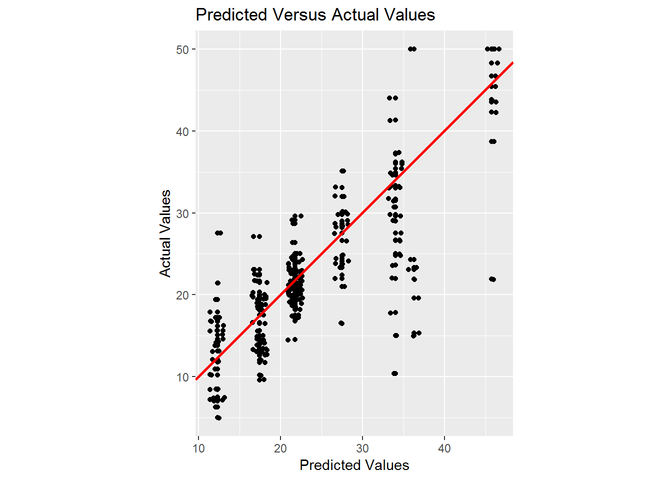
Based on this plot, it appears that we generally do a fairly good job estimating the average value of the actual values. We now calculate the average absolute error.
(avg_error <- sum(abs(test_predict - test_set[,14]))/length(test_predict))## [1] 3.707951So we can see that the average absolute error in our predictions is approximately 3.7079514. Overall, this error does not seem too bad. To reduce this error we could try including all of the variables from our dataset to see if we missed some other important variables.
In general, decision trees could be useful in determining the value of a house based on a variety of factors. A person looking to buy a house could even use this method to determine a good offer. You just need a good dataset and a little skill with R. In conclusion, decision trees are a really nice method which are easy to interpret and not too difficult to use.